Empirical validation of general relativity II: fundamental constants
Fundamental constants play a crucial (and perhaps surprising role) in the empirical tests of general relativity and the quest for modified gravity theories. Indeed, as we will discuss here:
- A space and/or time variation of the non-gravitational constants would be in direct violation with the Einstein Equivalence Principle (EEP). This would imply that gravitation can not be described by a metric theory of gravity and/or that a fifth fundamental interaction is required to describe fundamental physics.
- A space and/or time variation of the gravitational constant $G$ would be in direct violation with the Strong Equivalence Principle (SEP). This would imply that gravitation can not be described by a general relativity and that effectively a different metric would be required to describe the matter sector and the gravitational sector.
Fundamental constants: an overview
Inspired by the discussion of Uzan (2025), we can define the fundamental constants as the set of necessary parameters that cannot be explained by a theory, only measured. This definition covers several aspects:
- necessary: Fundamental constants are required, there is no way to get rid of them. They play key roles in a theory which can be different depending on the constant considered.
- cannot be explained/measured: The theory in which the constant appear cannot explain or derive their value anyhow. These values can only be measured. As such, the constant set clearly a theoretical limit of the theory.
- a theory: The number of fundamental constants depends on a given theory. As theories evolve, they can redefine the status and number of constants. One can hope that this number reduces with time, a signature that the theory has more and more explanatory power. Indeed, unificatory frameworks such as string theory might only need one fundamental (dimensional) constant (depending on who you ask), the string tension $T_S$. All the other constants of the standard model becoming byproducts of geometry or of field vacuum expectation values — and a constant which is secretly a field is free to vary.
Our standard model of particle physics together with general relativity requires 19 fundamental constants, listed in the table below. Ultimately, this number is expected to be even larger as the standard model does not account for observed phenomena such as the mass of neutrinos or dark matter.
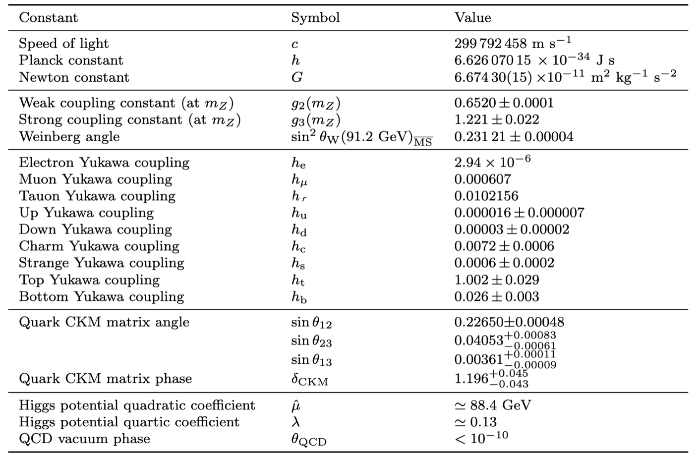
List of the fundamental constants for the standard model of particle physics and general relativity. Taken from Uzan (2025).
As a general matter of fact, we prefer to consider dimensionless parameters (as the fine-structure constant $\alpha$, see below), instead of constants with dimensions (such as $c$ and $\hbar$). The reason for this is that constants with dimensions can be interpreted as unit conversion factors instead of fundamental quantities. Dimensionless ratios, on the other hand, quantifies relationships between fundamental quantities. Indeed, it is always possible to fix $\hbar=c=1$ without changing the physics. Setting $\alpha=1$ would however give a theory in which the physics of the Universe is completely changed. Today, dimensional constants as $c$ are even fixed by convention in order to define unit systems (see again Uzan (2025) for a more detailed discussion).
Dimensionless constants of the standard models are of four broad types:
- Gauge couplings $g_i$, which quantify the relative strength of fundamental interactions. They can be also quantified through the fine structure constants defined as $\alpha_i = g_i^2/(4\pi)$ in natural units, which can be easier to measure.
- Yukawa couplings $h_i$ which quantify the masses of each particles (and are ultimately couplings of fermions with the Higgs boson). They can be measured directly by looking at mass ratios $m_i/m_j = h_i/h_j$.
- Symmetry breaking angles $\theta_i, \delta_{\rm CKM}$: which quantifies the breaking of symmetries as the terms of the CKM matrix and the strong vacuum phase, associated to the CP violations of the weak and strong forces respectively.
- Higgs Potential parameters, $\hat{\mu}$ and $\lambda$ defining the shape of the Higgs potential through the data of the mass of the Higgs boson and its quartic coupling respectively.
Non-gravitational constants and the EEP
We use the term “non-gravitational constants” here to describe broadly any fundamental constant that is not the Newton constant $G$ and that is not anyhow related to it.
A variation of the non-gravitational fundamental constants would lead to a direct violation of the local position invariance (LPI), which is one of the three building block of the EEP and that we defined in our previous class. Indeed, in such a case, the results of non-gravitational experimental tests would clearly depend on the region of space and time in which they are performed.
Furthermore, a space-time variation of the non-gravitational fundamental constants would lead to a violation of the weak equivalence principle (WEP) stating that all bodies must fall identically. This boils down to the fact that, if non-gravitational constants become dependent on space and time, so are the masses of the atoms and objects. We should not be surprised that several elements of the EEP are violated together by a variation of the constants, as this is exactly the statement of Schiff’s conjecture.
As we discussed in the previous lecture, the validity of the WEP is quantified by the value of the Eötvos parameter
\[\eta = 2\,\frac{|\vec{a}_1-\vec{a}_2|}{|\vec{a}_1+\vec{a}_2|}\]If we introduce the so-called sensitivity coefficient
\[f_i = \frac{\partial \ln(m_i)}{\partial \alpha}\]which quantifies how the mass $m_i$ of particle $i$ depends on a change of a non-gravitational constant $\alpha$.
It is then possible to show that, in a constant gravitational field $g$,
\[\boxed{\eta \simeq \frac{c^{2}}{g}\,|f_1-f_2|\,\big|\vec{\nabla}\alpha\big|}\]Thus measurements of the UFF also constraint varying non-gravitational constant models, and on the other hand, the variation of non-gravitational constant indeed induces a violation of the EEP.
The proof of this expression both in a Newtonian and in a general relativistic context can be found in the following bonus session.
Violation of WEP from varying constants
Consider any non-gravitational constant which we note $\alpha$. The mass of any composite body (e.g. an atom) depends on this constant, both through the masses of its constituents (yukawa couplings and Higgs potential) and through its internal binding energies (electromagnetic, strong, weak): $m = m(\alpha)$. If $\alpha$ becomes a function of space and time, $\alpha \to \alpha(x,t)$, this leads to a violation of the weak equivalence principle (WEP), i.e. of the universality of free fall. We show this first in Newtonian mechanics to build some intuition and then in general relativity.
The Newtonian version
Consider a particle of mass $m(\alpha)$ free-falling in the constant gravitational field $g$ of earth. We consider a Cartesian frame with unit vectors $\hat{x},\hat{y},\hat{z}=\hat{x_i}$. The particle is assumed to fall along the vertical $z$ axis, which is zero on the ground and pointing upward.
We start from the Lagrangian $L = T - V$ as the most fundamental quantity. In this context:
\[L = \frac{1}{2}m(\alpha)v^2 - m(\alpha)gz\]Here remember that $\alpha$ is a function of space and time and thus $m=m(\alpha(\vec{x},t))$. The Euler–Lagrange equations for each generalized coordinate $x_i$ are:
\[\frac{\text{d}}{\text{d}t}\frac{\partial L}{\partial \dot{x}_i}= \frac{\partial L}{\partial x_i}\]and in our context, only the one along the $z$ axis is non-trivial and gives:
\[\frac{\text{d}}{\text{d} t}\Big(m(\alpha)\,\dot{z}\Big) = \frac{\partial}{\partial z}\Big(\frac{1}{2}m(\alpha)\dot{z}^2 - m(\alpha)\,g z\Big),\]where the partial derivative is taken at fixed $\dot{z}$ and $t$. Expanding both sides and using the product rule we get:
\[\frac{\text{d} m}{\text{d} t}\dot{z} + m \ddot{z} = \frac{\partial m}{\partial z}\left(\frac{\dot{z}^2}{2} -gz\right) - mg\]where dotted quantities denote time derivatives (and $\text{d}m/\text{d}t = \partial_t m + \dot{z}\,\partial_z m$ is the total derivative along the trajectory). We thus notice additional terms that lead to a clear violation of the WEP. Indeed, if we rearrange the equation, we get:
\[\ddot{z}+g = -\frac{\text{d} \ln(m)}{\text{d} t}\dot{z} + \frac{\partial\ln(m)}{\partial z}\left(\frac{\dot{z}^2}{2} -gz\right)\]which should be strictly zero in standard Newtonian mechanics, for which $\ddot{z}=-g$ in agreement with WEP.
We can further develop this expression using the chain rule (recall that $m$ depends on $z$ and $t$ only through $\alpha$, with no explicit dependence):
\[\frac{\text{d}\ln(m)}{\text{d}t} = \frac{\partial \ln(m)}{\partial \alpha}\,\dot{\alpha}, \qquad \frac{\partial\ln(m)}{\partial z} = \frac{\partial \ln(m)}{\partial \alpha}\frac{\partial \alpha}{\partial z}\]where $\dot{\alpha} \equiv \text{d}\alpha/\text{d}t = \partial_t\alpha + \dot{z}\,\partial_z\alpha$ is the total derivative along the trajectory. We introduce the sensitivity coefficient:
\[f = \frac{\partial \ln(m)}{\partial \alpha}\]The important aspect is that $f$ will be different depending on the particle under consideration. For example different atoms will have different number of protons and electrons and thus will depend differently on the non-gravitational constants, like the fine-structure constant. The general expression to get the mass of an atom in terms of the mass of its constituants and their interactions is known as the Bethe-Weizsäcker formula.
Now, it is quite straightforward to generalize the previous expression to vector form:
\[\vec{a}-\vec{g}= -f\dot{\alpha}\,\vec{v}+ f\vec{\nabla}\alpha\left(\frac{v^2}{2}- \Phi\right)\]where $\Phi = gz$ is the gravitational potential. If we add the rest-mass term $L_0 = -mc^2$ to the Lagrangian (the leading term of the non-relativistic expansion $-mc^2\sqrt{1-v^2/c^2}\approx -mc^2 + \frac{1}{2}mv^2$), we obtain the final expression:
\[\boxed{\vec{a}-\vec{g}= -f\dot{\alpha}\,\vec{v}+ f\vec{\nabla}\alpha\left(-c^2+\frac{v^2}{2}- \Phi\right)}\]Now consider two particles with masses $m_1$ and $m_2$ and sensitivity coefficients $f_1$ and $f_2$, compared at the same point with the same velocity $\vec{v}$. They fall differently, leading to a non-zero value of the so-called Eötvös parameter
\[\eta = 2\,\frac{|\vec{a}_1-\vec{a}_2|}{|\vec{a}_1+\vec{a}_2|}\]From the formula above, using $\vert\vec{a}_1+\vec{a}_2\vert \approx 2g$, $\vec{v}_1 \simeq \vec{v}_2$ and $\alpha_1 \simeq \alpha_2$, we get directly
\[\eta \simeq \frac{|f_1-f_2|}{g}\left|\,\dot{\alpha}\,\vec{v} + \vec{\nabla}\alpha\left(c^{2}-\frac{v^{2}}{2}+\Phi\right)\right|\]and hence
\[\boxed{\eta \simeq \frac{c^{2}}{g}\,|f_1-f_2|\,\big|\vec{\nabla}\alpha\big|}\]since the rest-mass contribution dominates by a factor $\sim c^2/v^2$.
In General relativity
In General relativity, the action of a point-like particle with a $\alpha$ dependent mass is given by
\[S = -\int m(\alpha) \text{d}s = -\int m(\alpha) \sqrt{-g_{\mu\nu}u^\mu u^\nu} \text{d}\tau\]with $u^\mu = \text{d}x^\mu / \text{d}\tau$ and $\tau$, the proper time, is used to parametrize the curve of the massive particle.
This action leads to the geodesic equation $u^\nu\nabla_\nu u^\mu =0$ when extremalized if $m$ is constant. If $m$ varies, we obtain
\[\boxed{u^\nu\nabla_\nu u^\mu = -f \partial_\beta \alpha \left(g^{\beta\mu} + u^{\beta}u^\mu\right)}\]Hence, the space-time variation of $\alpha$ will deviate geodesics in a component dependent way (as $f$ is different depending on the atom under consideration).
Proof: The derivation follows identical step as the standard geodesic equation we derived in our first class, with extra-terms. The first term remains unchanged:
\[\frac{\partial L}{\partial \dot x^\beta} =\frac{m}{\sqrt{-\vert u \vert^2}}\,g_{\beta\alpha}\dot x^\alpha\]but the second term gets derivative of the mass term:
\[\begin{align} \frac{\partial L}{\partial x^\beta} = \frac{m}{2\sqrt{-\vert u \vert^2}}\,\partial_\beta(g_{\mu\nu})\,\dot x^\mu\dot x^\nu - \frac{\partial m}{\partial x^\beta}\sqrt{-\vert u \vert^2}, \end{align}\]We should also not forget the derivative with respect to $\tau$ of the mass when putting everything together in the Lagrange equation:
\[\frac{\text{d}m}{\text{d}\tau} \frac{1}{\sqrt{-\vert u \vert^2}}\,g_{\beta\alpha}\dot x^\alpha + m\frac{\text{d}}{\text{d}\tau}\left(\frac{1}{\sqrt{-\vert u \vert^2}}\,g_{\beta\alpha}\dot x^\alpha\right) - \frac{m}{2\sqrt{-\vert u \vert^2}}\,\partial_\beta(g_{\mu\nu})\,\dot x^\mu\dot x^\nu + \frac{\partial m}{\partial x^\beta}\sqrt{-\vert u \vert^2}=0\]Hence, considering a trajectory along which $\vert u^2\vert=-1$, we get:
\[u^\mu \nabla_\mu u_\alpha = -\frac{\text{d}\ln(m)}{\text{d}\tau}u_\alpha - \frac{\partial \ln(m)}{\partial x^\alpha}\]Along the worldline the chain rule gives $\frac{\text{d}\ln m}{\text{d}\tau} = u^\sigma \partial_\sigma \ln m$, so both terms carry the same factor $\partial_\sigma \ln m$ and can be combined:
\[u^\mu \nabla_\mu u_\alpha = -\partial_\sigma \ln m(u^\sigma u_\alpha + \delta^\sigma_\alpha)\]Writing $\partial_\sigma \ln m= f \partial_\sigma \alpha$ and raising the free index with the metric, we get as desired:
\[u^\nu\nabla_\nu u^\mu = -f \partial_\beta \alpha \left(g^{\beta\mu} + u^{\beta}u^\mu\right)\]Newtonian limit: Taking the Newtonian limit that we now know very well, the $\mu=i$ components of the left-hand side give \(\frac{\text{d}^2x^i}{\text{d}t^2} + \partial^i\Phi\). For the right-hand side, we easily find \(-f\,\partial_t\alpha\left(g^{0i}+u^0u^i\right) - f\,\partial_j\alpha\left(g^{ji}+u^ju^i\right)\)
We set ourselves in the Newtonian gauge $g^{0i}=0$ and $g^{ij}\simeq\delta^{ij}$, while at leading order $u^0\simeq 1$ and $u^i\simeq v^i$, such that the right hand side becomes:
\[\text{R.H.S.}\simeq -f\,(\partial_t\alpha)\,v^i - f\,\partial^i\alpha - f\,v^iv^j\partial_j\alpha = -f\,v^i\underbrace{\left(\partial_t\alpha + v^j\partial_j\alpha\right)}_{\displaystyle \dot\alpha} - f\,\partial^i\alpha\]Restoring $c$ and writing in vector form, the full equation is:
\[\vec{a}-\vec{g} = -f\dot{\alpha}\,\vec{v} - c^2 f\,\vec{\nabla}\alpha\]which is exactly the Newtonian result obtained above, up to the relative correction $\left(\frac{v^2}{2}-\Phi\right)/c^2 \ll 1$ which would be an higher order refinement. The two derivations therefore agree at the order to which both are truncated, and in particular give the same Eötvös parameter dominated by the mass term.
The fine structure constant
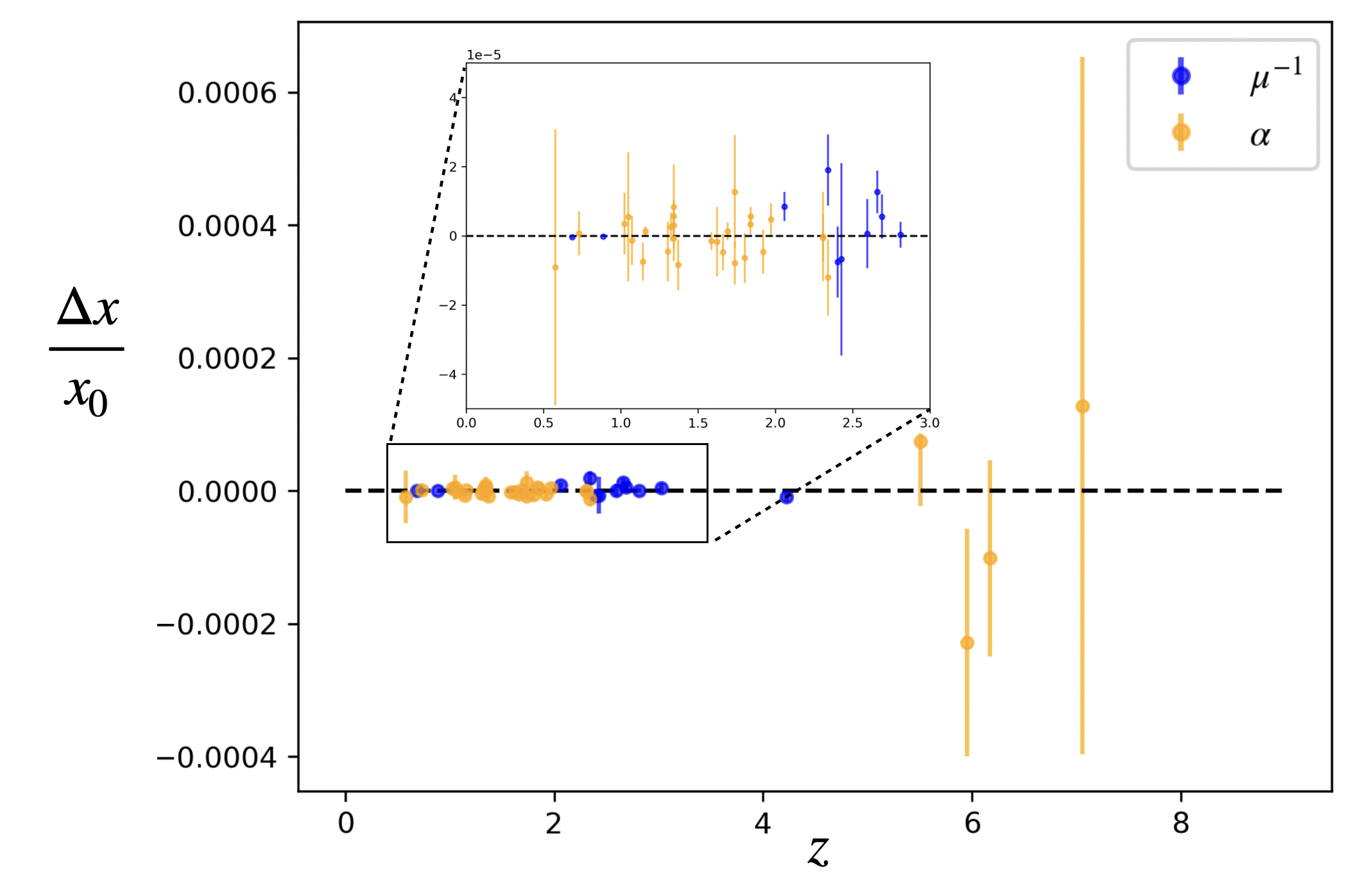
Figure 1: Measurement from QSO of varying constants. Data taken from Uzan (2025).
Amongst all the non-gravitational constants, two are of primary interest when looking for variations in space and time: the fine-structure constant $\alpha$ and the electron-to-proton mass ratio $\mu \equiv m_e/m_p$. The reason is that between them they govern essentially the whole of atomic and molecular spectroscopy, which is the only information we ever receive from distant objects.
The fine-structure constant sets the strength of electromagnetism relative to the other interactions. There is a simple way to see this without invoking any sophisticated concept. Expressing the charges of two objects as multiples $z_1, z_2$ of the elementary charge and working in natural units $\hbar = c = 1$, the Coulomb force reads
\[\vec{F}_C = \frac{\alpha\, z_1 z_2}{r^2}\,\hat{r}\]Compare this with Newton’s law $\vec F_N = G m_1 m_2 / r^2$: $\alpha$ plays for electromagnetism exactly the role that $G$ plays for gravity — it is the coupling constant that converts a product of charges into a force. The essential difference is that $\alpha$ is dimensionless whereas $G$ is not (and this has deep implication for the possibility to build a quantum theory of gravity).
In S.I. units:
\[\boxed{\alpha = \frac{e^2}{4\pi \hbar c\varepsilon_0}}\]$\alpha =7.297 352 5643 (11) \times 10^{-3} \simeq 1/137$ (from CODATA). Note the relative precision of $1.6\times10^{-10}$ — one of the best-measured numbers in physics. If $\alpha$ were different by a few $\%$, the Universe as we know it would be completely altered. A significantly higher $\alpha$ would make chemistry impossible, as atoms would not be able to share electrons as easily as they do. A significantly lower $\alpha$ on the other hand, would prevent electrons to bound with nuclei to form atoms, and all the matter in the Universe would remain as a plasma.
In the quest for EEP violations on various scale, we consider the fine-structure constant as a fantastic target, for a combination of theoretical and observational reasons:
-
It is fundamental, and yet tied to very familiar physics. It appears in the Bohr energy levels, in the Compton and Thomson cross-sections, in the quantum electrodynamics (QED) perturbative expansion — one does not need exotic machinery to know what a shift in $\alpha$ would do.
-
It controls very precise quantum transitions. The atomic energy levels used as probes involve only QED, a theory known to extraordinary accuracy and perturbatively tractable. This is a decisive practical advantage over constants entering through quantum chromodynamics (QCD), where the relation between the fundamental parameters and the observable (a nuclear binding energy, say) requires non-perturbative modelling and carries large theoretical uncertainties.
-
It governs light itself. Electromagnetic radiation remains our primary and, in most cases, only probe of astrophysical objects. A constant imprinted directly on photon emission and absorption is therefore measurable arbitrarily far away in both space and time — something that cannot be said of most other parameters of the Standard Model.
The available constraints on $\alpha$ span an enormous range in time, allowing to strongly constraint any models which would predict a violation of the EEP across cosmic history.
Atomic clocks ($z = 0$). The most direct approach: compare two clock transitions with different sensitivities to $\alpha$ over several years and look for a relative drift. Operating a single $^{171}$Yb$^+$ ion clock and interleaving the electric octupole (E3) transition — highly sensitive to $\alpha$ — with the electric quadrupole (E2) transition, Filzinger et al. (2023) obtain
\[\frac{\dot\alpha}{\alpha_0} = (1.8 \pm 2.5)\times10^{-19}\ {\rm yr^{-1}}\]This is a constraint on the present-day drift rate only; extrapolating it backwards assumes a linear evolution, which no realistic model predicts.
The Oklo natural reactor ($z \simeq 0.14$, $\sim 1.8$ Gyr ago). Around two billion years ago, when the first eukaryotic cells were appearing on Earth, a uranium deposit in Gabon reached criticality and operated as a natural fission reactor. The isotopic abundances left behind are exquisitely sensitive to the position of a 97.3 meV neutron capture resonance in $^{149}$Sm, which in turn depends on $\alpha$. Using realistic MCNP models of the RZ2 and RZ10 reactor zones, Gould, Sharapov & Lamoreaux (2006) obtain $-1.1\times10^{-8} < \Delta\alpha/\alpha_0 < 2.4\times10^{-8}$, i.e.
\[\frac{\Delta\alpha}{\alpha_0} = (0.65 \pm 1.75)\times10^{-8}\]This is numerically the tightest bound at non-zero redshift, but it depends heavily on the reactor model adopted and on the fine details of the nuclear physics involved — the same authors showed that earlier disagreements in the literature traced back entirely to different assumed neutron spectra. It should be treated with more caution than its formal error bar suggests.
Quasar absorption spectra ($0.2 \lesssim z \lesssim 4$). Light from a distant supermassive black-holes, the quasars (quasi stellar objects, QSO), passes through intervening gas clouds, which imprint absorption lines at the redshift of the cloud. Comparing the relative spacing of many transitions with different sensitivity coefficients — the Many-Multiplet method — isolates a shift in $\alpha$ from the overall Doppler shift. Indeed while doppler shift has a linear effect on the transition line (it shift them rigidly), varying $\alpha$ Current data reach the part-per-million (ppm) level out to $z\sim 3$ and are summarised in Figure 1. A historically influential claim of a spatial dipole in $\alpha$ has since been largely attributed to wavelength-calibration systematics; modern instruments designed for this purpose give null results at the ppm level.
Early universe ($z \sim 10^3$ and $z\sim10^8$). The CMB alone, or in addition with other cosmological probes (breaking degeneracies) allow to reach a constraint on $\alpha$ at recombination at the $\sim10^{-3}$ level. More precisely, one reaches \(\frac{\Delta \alpha}{\alpha_0}= 0.037 ± 0.17 \%\) for the CMB alone (Planck + ACT) and reaches \(0.043 ± 0.17 \%\) adding the BAO data Calabrese (2025). So far, this is the oldest almost direct measurement one can do of the fundamental constants in the Universe, as this is the oldest light one can observe. Other even older constraints can be derived from the Big bang nucleosynthesis (BBN), but, as for the Oklo bound, the results are very dependent on the details of the nuclear processes at stake as well as the phenomenological model used (as possible co-variations of constants).
| Probe | Epoch | Quantity | Constraint |
|---|---|---|---|
| Atomic clocks | $z=0$ | $\dot\alpha/\alpha_0$ | $(1.8\pm2.5)\times10^{-19}\ \rm yr^{-1}$ |
| Oklo reactor | $z\simeq0.14$ | $\Delta\alpha/\alpha_0$ | $(0.65\pm1.75)\times10^{-8}$ |
| QSO absorption | $0.2\lesssim z\lesssim4$ | $\Delta\alpha/\alpha_0$ | $\sim10^{-6}$ |
| CMB | $z\simeq1100$ | $\Delta\alpha/\alpha_0$ | $\sim10^{-3}$ |
The electron to proton mass ratio
Another very relevant dimensionless constant is the electron to proton mass ratio:
\[\mu = \frac{m_e}{m_p}\]Depending on the experiment, or the theoretical framework, it is also frequent to consider its inverse:
\[\overline{\mu}= \mu^{-1} = \frac{m_p}{m_e}\]which is measured to be $\overline{\mu}=1836.152 673 426(32)$ from CODATA. In other word: the proton is $\sim 1840$ times heavier than the electron, and there is no way for our fundamental theories to explain why. The formation of atoms rely heavily on this mass difference, and the Universe would be drastically different if $\mu$ had a significantly different value.
Similarly to $\alpha$, it is possible to give very precise measurements of $\mu$ using spectroscopy (the bounds based on nuclear processes such as Oklo or BBN can not apply here, as the electron has nothing to do with the physics of nuclei).
Mostly we have:
Atomic clocks ($z = 0$).: Similarly to the atomic clocks measurement of $\alpha$, allow to obtain the stringent bound on the time variation of $\mu$:
\[\frac{\dot{\mu}}{\mu_0} = (3.09 \pm 1.42)\times 10^{-17} \, {\rm yr^{-1}}\]Quasar absorption spectra ($0.2 \lesssim z \lesssim 4$). Similary to $\alpha$, clouds absorption lines of QSO light are sensitive to the value of $\overline{\mu}$ at different redshift. The measurements can be found on Figure 1.
Early universe ($z \sim 10^3$). CMB allows to constrain $\mu$ at the percent level, reaching fraction of a percent in combination with other cosmological data sets. More precisely, \(\frac{\Delta \mu}{\mu_0}= 14.4^{+6}_{-7.3}\%\) for the CMB alone (Planck + ACT) and \(\frac{\Delta \mu}{\mu_0}= 0.96 \pm 0.6\%\) adding the BAO data (Calabrese (2025)).
Gravitational constant and the SEP
While this might sound obvious, let us stress that the gravitational constant $G$ plays a very special role regarding gravity and its tests. Indeed, it is the only fundamental constant of general relativity (along with the cosmological constant $\Lambda$, which could arguably deserve such a title1): $G$ quantifies the strength of gravity. As we teased multiple times already in this lecture, a space-time variation of $G$ would imply a violation of the strong equivalence principle (SEP) — a principle which GR might well be the only theory to satisfy (at least the only empirically viable one, see our later discussion of Nordström’s theory).
Unfortunately, gravity is an extremely weak force and always appears to us as a classical phenomenon. Measuring $G$ is therefore much more difficult than measuring non-gravitational constants such as the fine-structure constant $\alpha$ or the proton-to-electron mass ratio $\mu$, which are tied to sharp quantum predictions like atomic lines. The current recommended value, $G=6.67430(15) \times 10^{-11}$ m$^{3}\,$kg$^{-1}\,$s$^{-2}$ (CODATA 2022), carries a relative uncertainty of $2.2\times 10^{-5}$ — by far the worst of all fundamental constants ($\alpha$ is known to $10^{-10}$). Worse, independent laboratory (Cavendish-type) measurements disagree with each other by up to $\sim 5\times 10^{-4}$, well beyond their quoted uncertainties — the so-called “big $G$ problem”. For more on this, see e.g. Gibney (2026).
Why is the gravitational force so weak?
The strength of interactions of the standard models are quantified by dimensionless parameters, known as fine-structure constants $\alpha_i = g_i^2/(4\pi\hbar c)$, where $g_i$ is the coupling associated to the force (appearing in the covariant derivatives of the fermion fields). In order to compare gravity with other forces, it is possible to define an equivalent gravitational fine-structure constant as follows:
\[\boxed{\alpha_G = \frac{Gm_p^2}{\hbar c} = \left(\frac{m_p}{m_{\rm Pl}}\right)^2 \simeq 5.9\times 10^{-39}}\]where $m_{\rm Pl}=\sqrt{\hbar c/G}\simeq 1.2\times 10^{19}$ GeV$/c^2$ is the Planck mass. Compare with the strong, weak and electromagnetic fine structure constants: $\alpha_S \sim 0.12$, $\alpha_W \sim 0.03$, $\alpha \simeq 1/137 \sim 0.007$. Gravity is weaker by almost forty orders of magnitude — equivalently, the proton is absurdly light compared to the Planck mass. Why the electroweak scale ($\sim 10^2$ GeV) sits seventeen orders of magnitude below the Planck scale, and why quantum corrections do not drag it back up, is an easy version of the complicated hierarchy problem, one of the main open questions of particle physics today.
To propose a solution to this problem and explain the mysterious values of the constants, it was first proposed by Dirac (1937) that $G$ could evolve with cosmic time. This is the first known “varying constant” proposal in modern physics. Dirac noticed a curious coincidence: the ratio of the electric to the gravitational force between a proton and an electron, $N_1 = e^2/(4\pi\varepsilon_0 G m_p m_e) \sim 10^{39}$, is comparable to the age of the Universe expressed in atomic units, $N_2 = t_0/(e^2/4\pi\varepsilon_0 m_e c^3) \sim 10^{39}$. Refusing to see such enormous pure numbers as accidental, he postulated $N_1 \propto t$, i.e. $G \propto 1/t$, predicting $\dot G/G \simeq -H_0 \sim -7\times 10^{-11}$ yr$^{-1}$. The idea is wrong — we will see below that such a drift is excluded by more than four orders of magnitude — but it is historically important: it launched the entire field of varying-constants phenomenology (see also Feynman’s Lectures on Gravitation). Two classic rebuttals deserve mention. Teller (1948) noted that the solar luminosity depends steeply on $G$ ($L_\odot \propto G^7$ roughly, at fixed mass): with Dirac’s law the Sun would have boiled the oceans in the Cambrian era, contradicting the most recent discoveries of paleontology. Dicke (1961) later dissolved the coincidence with what can be understood as an anthropic argument: observers exist only during the stellar-burning epoch, whose duration is itself fixed by $\alpha_G$ — so $N_1\sim N_2$ is expected to happen if some observers exist to witness it. anthropic arguments to explain the values of fundamental constants have since then been invoked multiple times in order to explain why the constants of the Universe seems to be so fine tuned in order to allow for the emergence of conscious life. Our Universe might be only one “lucky” random draw in a multitude of inhospitable universes with different constants.
Varying gravitational constant
As stated earlier in this lecture, dimensionless numbers are unambiguously measurable: a claimed variation of a dimensionful constant can be undone by a redefinition of units (Uzan 2024). A variation of $G$ is thus better understood as a variation of $\alpha_G = (m_p/m_{\rm Pl})^2$: hence, saying that $G$ grows is strictly equivalent to saying that all particle masses shrink identically in Planck units. What distinguishes it from a variation of $\alpha$ or $\mu$ is that it affects all masses universally — which is precisely why it violates the SEP and not the EEP. Indeed, it is thus possible to satisfy the EEP while violating the SEP — and in fact many modified-gravity theories are designed to do just that: matter couples minimally to the metric (EEP holds, weak-field tests passed), but the gravitational “constant” is promoted to a dynamical field (SEP violated). We will come back to this with a concrete example when discussing the Brans-Dicke theory.
Hence, as further discussed in the two following complements, a varying $G$ implies that different (effective) metric are present in the gravitational and in the matter Lagrangian. Furthermore, it also implies that gravity does not gravitate universally and thus that one would observe some Nordtvedt effect in a varying $G$ theory. For some more details on this, have a look at the following supplement.
Varying $G$, violation of the SEP and Nordtvedt effect
Recall that the SEP extends the EEP by two clauses: (i) the universality of free fall holds also for self-gravitating bodies, and (ii) local gravitational experiments (not just non-gravitational ones) are insensitive to where, when, and at which velocity they are performed. Clause (ii) is local position invariance (LPI) and local Lorentz invariance (LLI) applied to gravity itself.
“A varying $G$” is, by definition, a violation of clause (ii). Indeed, by the EEP, all matter couples to a single metric $g$: rods, clocks and particle masses are built from \(\mathcal{L}_m(\psi,g)\) and are constant in matter units. The statement “$G$ varies” then has only one operational meaning: the dimensionless outcome \(\alpha_G = G_{\rm eff}m_p^2/\hbar c\) of a local gravitational (Cavendish-type) experiment differs from one space-time event to another. But this is precisely a violation of LPI for a gravitational experiment — clause (ii) of the SEP. The implication “varying $G$ $\Rightarrow$ SEP violation” therefore holds with no assumption whatsoever about the underlying theory. Note however, that all “non-gravitational” experiments remain untouched by such a variation of $G$, and hence the LPI and LLI remain untouched by a varying $G$.
It also violates (i), perhaps unsurprisingly (the connection between the two is expected to be almost always satisfied as stated by a strong version of the Schiff conjecture). Taking a body \(A\) of mass $m_A$. It is expressed as \(m_Ac^2 = m_0c^2 + E_{\text{int}} + E_g\), where $m_0$ is the mass of all constituents including non-gravitational binding energies, $ E_{\text{int}}$ is its internal energy and $E_g$ is the gravitational binding energy. For a body of mass density $\rho$, $E_g = - \int (Gm(r)\rho(r))/r\text{d}r$, containing $G$. The internal energy $E_{\text{kin}}$ of the body (as a star) can also depends on $G$ (and even could some kinetic energy due to rotation). In short: $G$ drives all of the energy budget of a self gravitating bodies. Hence, masses of self-gravitating objects varies with $G$. Following exactly the same argument as the one for non-gravitational constants (above), this implies a violation of the universality of free-fall for two bodies with different gravitational binding energies, and hence different dependence of $m_A$ in $G$. This is the definition of the Nordtvedt effect, introduced in the previous lecture and thus in specific theories, constraints on $\eta_N$ can be translated on constraints on varying $G$. However, for small test bodies, self gravitational binding energy is totally negligible. Bodies might fall on different geodesics than in GR (due to the variation of $G$), but they will all follow the same trajectories, independently of their composition. Hence, the WEP is satisfied and by extension the EEP. A theory with a varying $G$ is hence metric but violates the SEP.
As we discussed in our first lecture, the SEP implies that the two metrics appearing in the gravitational and matter Lagrangians are the same. Hence: a theory with varying $G$ is necessarily of the form
\[S = S_{\rm grav}[g^*, \phi^a] + S_m[\psi;\, g], \qquad g = g[g^*,\phi^a],\]i.e. the metric \(g^*\) of the gravitational Lagrangian (the one with constant couplings) is not the metric $g$ felt by matter, the two being bridged by additional fields $\phi^a$ mediating gravity. We prove formally the equivalence between a varying $G$ and this difference of metric below. As long as there is a unique $g$ coupling to matter, and not a $g_i$ for different matter type, the EEP is satisfied and the theory is metric. Hence, the field $\phi^a$ must couple only to gravity, or equivalently it should couple identically to all matter fields. In such a case, the theory is metric, but $G$ varies. The locally measured $G$ is then a function of the local background values $\phi^a_0$; and these are fixed not by the laws of physics but by boundary conditions — the cosmological history of $\phi^a$ and the surrounding matter distribution. We will come back to the simplest theories of varying $G$ in a later class on the Brans-Dicke model. For a discussion of forms for the function relating \(g^*,\phi\) and $g$, see also e.g. Bekenstein (1992) and Damour and Esposito-Farese (1991).
Let us now proove why a varying $G$ theories is equivalent to a theory with two metrics. Imagine that our theory is general relativity, with a varying $G$, which should be, or depend on some fields $\phi^a$ in order to be self-consistent. These fields must also be described by their own Lagrangian \(\mathcal{L}_\phi[\phi^a;\, g]\). The total and most general action of General relativity with varying $G$ is thus:
\[S = \int d^4x\,\sqrt{-\vert g\vert}\left(\frac{R[g]}{16 \pi G(\phi^a)} + \mathcal{L}_\phi[\phi^a;\, g] + \mathcal{L}_m[\psi;\, g]\right).\]The claim is that this is identically a theory with two metrics: one with a constant gravitational coupling in the gravitational sector, and a different one in the matter sector.
First, let’s absorb $G(\phi^a)$ into a new metric. Let $G_0$ be the value of $G(\phi^a)$ today, and define
\[g^*_{\mu\nu} \equiv \frac{G_0}{G(\phi^a)}\, g_{\mu\nu} \qquad\Longleftrightarrow\qquad g_{\mu\nu} = A^2(\phi^a)\, g^*_{\mu\nu}, \quad A^2 \equiv \frac{G(\phi^a)}{G_0}.\]This is a mere field redefinition — a change of variables $(g,\phi^a)\to(g^*,\phi^a)$, with no physical content — and it requires only $G>0$. Such a transformation of \(g \to g^*\) is called a conformal transformation, as it changes all the length but not the angles. We will encounter them all over again in these classes.
We can now transform the curvature term. In 4 dimensions, the conformal rescaling \(g = A^2 g^*\) obeys \(\sqrt{-\vert g\vert} = A^4\sqrt{-\vert g^*\vert}\) and \(R[g] = A^{-2}\left(R[g^*] - 6\,\Box_* \ln A - 6\,(\partial \ln A)^2_*\right)\).
Proof of the relation involving the curvature
Throughout, starred quantities (\(\Gamma^*\), \(\nabla^*\), \(\Box_*\), \(R^*\)) are built from \(g^*\), and indices are raised/lowered with \(g^*\). It is convenient to write \(A = e^{\omega}\), i.e. \(\omega \equiv \ln A\). This rewritting will simplify our calculations enormously. Using it, we find that \(g_{\mu\nu} = e^{2\omega} g^*_{\mu\nu}\) and \(g^{\mu\nu} = e^{-2\omega} g^{*\mu\nu}\). As a reminder \(\Box_* = g^*_{\mu\nu}\partial^\mu \partial^\nu\).
First, we rederive the formula for the volume element. In 4 dimensions, \(\det(g) = \det(e^{2\omega}g^*) = (e^{2\omega})^4 \det(g^*)\), hence
\[\sqrt{-\vert g\vert} = e^{4\omega}\sqrt{-\vert g^*\vert} = A^4 \sqrt{-\vert g^*\vert}.\]Now, we look at the difference between the Christoffel symbols, that will ultimately appear in the expression of the Riemann tensor and the Ricci scalar. Insert the rescaling into \(\Gamma^{\rho}_{\mu\nu} = \tfrac{1}{2}g^{\rho\sigma}\left(\partial_\mu g_{\sigma\nu} + \partial_\nu g_{\sigma\mu} - \partial_\sigma g_{\mu\nu}\right)\), using \(\partial_\mu g_{\sigma\nu} = e^{2\omega}\left(\partial_\mu g^*_{\sigma\nu} + 2\,\partial_\mu\omega\; g^*_{\sigma\nu}\right)\). The factors \(e^{-2\omega}\) from \(g^{\rho\sigma}\) and \(e^{2\omega}\) from the derivatives cancel. We then obtain:
\[\Gamma^{\rho}_{\mu\nu} = \Gamma^{*\rho}_{\mu\nu} + g^{*,\rho\sigma}\left(\partial_\mu \omega g^{*}_{\sigma \nu} + \partial_\nu \omega g^{*}_{\sigma \mu} - \partial_\sigma \omega g^{*}_{\mu \nu}\right)\]From which we can write (recall that \(g^{\mu\rho}g_{\rho\nu} = \delta^\mu_\nu\) by definition of the inverse metric):
\[C^{\rho}{}_{\mu\nu} \equiv \Gamma^{\rho}_{\mu\nu} - \Gamma^{*\rho}_{\mu\nu} = \delta^{\rho}_{\mu}\,\partial_\nu\omega + \delta^{\rho}_{\nu}\,\partial_\mu\omega - g^*_{\mu\nu}\,\partial^{\rho}\omega .\]Note that it is possible to show that \(C^{\rho}{}_{\mu\nu}\) is a tensor (difference of two connections), so it may be manipulated covariantly. Its trace will be needed: contracting \(\rho\) with \(\mu\),
\[C^{\rho}{}_{\nu\rho} = \partial_\nu\omega + 4\,\partial_\nu\omega - \partial_\nu\omega = 4\,\partial_\nu\omega .\]Insert \(\Gamma = \Gamma^* + C\) into the definition of the Riemann tensor \(R^{\rho}{}_{\sigma\mu\nu} = \partial_\mu \Gamma^{\rho}{}_{\nu\sigma} - \partial_\nu \Gamma^{\rho}{}_{\mu\sigma} + \Gamma^{\rho}{}_{\mu\lambda}\Gamma^{\lambda}{}_{\nu\sigma} - \Gamma^{\rho}{}_{\nu\lambda}\Gamma^{\lambda}{}_{\mu\sigma}.\) The terms quadratic in \(\Gamma^*\) and the \(\partial\Gamma^*\) terms reassemble \(R^{*\rho}{}_{\sigma\mu\nu}\); the cross terms \(\Gamma^* C\) combine with \(\partial C\) into covariant derivatives of \(C\); the terms quadratic in \(C\) remain. The result is the exact identity
\[R^{\rho}{}_{\sigma\mu\nu} = R^{*\rho}{}_{\sigma\mu\nu} + \nabla^*_{\mu}C^{\rho}{}_{\nu\sigma} - \nabla^*_{\nu}C^{\rho}{}_{\mu\sigma} + C^{\rho}{}_{\mu\lambda}C^{\lambda}{}_{\nu\sigma} - C^{\rho}{}_{\nu\lambda}C^{\lambda}{}_{\mu\sigma}.\]where we recall that \(\nabla^*_{\mu}C^{\rho}{}_{\nu\sigma} = \partial_\mu C^{\rho}{}_{\nu\sigma}+ \Gamma^{*\rho}{}_{\mu\lambda}\,C^{\lambda}{}_{\nu\sigma} - \Gamma^{*\lambda}{}_{\mu\nu}\,C^{\rho}{}_{\lambda\sigma}- \Gamma^{*\lambda}{}_{\mu\sigma}\,C^{\rho}{}_{\nu\lambda}\,\). Contracting \(\rho\) with \(\mu\):
\[R_{\sigma\nu} = R^*_{\sigma\nu} + \nabla^*_{\rho}C^{\rho}{}_{\nu\sigma} - \nabla^*_{\nu}C^{\rho}{}_{\rho\sigma} + C^{\rho}{}_{\rho\lambda}C^{\lambda}{}_{\nu\sigma} - C^{\rho}{}_{\nu\lambda}C^{\lambda}{}_{\rho\sigma}.\]Let’s now evaluate the four terms. With our expression for \(C\) (and using \(\nabla^*_\mu\partial_\nu\omega = \nabla^*_\nu\partial_\mu\omega\) on a scalar):
(a) \(\nabla^*_{\rho}C^{\rho}{}_{\nu\sigma} = \nabla^*_{\nu}\partial_{\sigma}\omega + \nabla^*_{\sigma}\partial_{\nu}\omega - g^*_{\nu\sigma}\Box_*\omega = 2\nabla^*_{\nu}\nabla^*_{\sigma}\omega - g^*_{\nu\sigma}\,\Box_*\omega .\)
(b) \(\nabla^*_{\nu}C^{\rho}{}_{\rho\sigma} = 4\,\nabla^*_{\nu}\nabla^*_{\sigma}\omega .\)
(c) \(C^{\rho}{}_{\rho\lambda}C^{\lambda}{}_{\nu\sigma} = 4\,\partial_\lambda\omega\left(\delta^{\lambda}_{\nu}\partial_\sigma\omega + \delta^{\lambda}_{\sigma}\partial_\nu\omega - g^*_{\nu\sigma}\partial^{\lambda}\omega\right) = 8\,\partial_\nu\omega\,\partial_\sigma\omega - 4\,g^*_{\nu\sigma}(\partial\omega)^2_* .\)
(d) The last term requires care. Writing out both factors,
\[C^{\rho}{}_{\nu\lambda} = \delta^{\rho}_{\nu}\partial_\lambda\omega + \delta^{\rho}_{\lambda}\partial_\nu\omega - g^*_{\nu\lambda}\partial^{\rho}\omega, \qquad C^{\lambda}{}_{\rho\sigma} = \delta^{\lambda}_{\rho}\partial_\sigma\omega + \delta^{\lambda}_{\sigma}\partial_\rho\omega - g^*_{\rho\sigma}\partial^{\lambda}\omega,\]the product contracted over \(\rho\) and \(\lambda\) has nine terms:
| term | value |
|---|---|
| \(\delta^{\rho}_{\nu}\partial_\lambda\omega \cdot \delta^{\lambda}_{\rho}\partial_\sigma\omega\) | \(+\,\partial_\nu\omega\,\partial_\sigma\omega\) |
| \(\delta^{\rho}_{\nu}\partial_\lambda\omega \cdot \delta^{\lambda}_{\sigma}\partial_\rho\omega\) | \(+\,\partial_\nu\omega\,\partial_\sigma\omega\) |
| \(\delta^{\rho}_{\nu}\partial_\lambda\omega \cdot (-g^*_{\rho\sigma}\partial^{\lambda}\omega)\) | \(-\,g^*_{\nu\sigma}(\partial\omega)^2_*\) |
| \(\delta^{\rho}_{\lambda}\partial_\nu\omega \cdot \delta^{\lambda}_{\rho}\partial_\sigma\omega\) | \(+\,4\,\partial_\nu\omega\,\partial_\sigma\omega\) |
| \(\delta^{\rho}_{\lambda}\partial_\nu\omega \cdot \delta^{\lambda}_{\sigma}\partial_\rho\omega\) | \(+\,\partial_\nu\omega\,\partial_\sigma\omega\) |
| \(\delta^{\rho}_{\lambda}\partial_\nu\omega \cdot (-g^*_{\rho\sigma}\partial^{\lambda}\omega)\) | \(-\,\partial_\nu\omega\,\partial_\sigma\omega\) |
| \((-g^*_{\nu\lambda}\partial^{\rho}\omega) \cdot \delta^{\lambda}_{\rho}\partial_\sigma\omega\) | \(-\,\partial_\nu\omega\,\partial_\sigma\omega\) |
| \((-g^*_{\nu\lambda}\partial^{\rho}\omega) \cdot \delta^{\lambda}_{\sigma}\partial_\rho\omega\) | \(-\,g^*_{\nu\sigma}(\partial\omega)^2_*\) |
| \((-g^*_{\nu\lambda}\partial^{\rho}\omega) \cdot (-g^*_{\rho\sigma}\partial^{\lambda}\omega)\) | \(+\,\partial_\nu\omega\,\partial_\sigma\omega\) |
Summing: \(C^{\rho}{}_{\nu\lambda}C^{\lambda}{}_{\rho\sigma} = 6\,\partial_\nu\omega\,\partial_\sigma\omega - 2\,g^*_{\nu\sigma}(\partial\omega)^2_* .\)
Now for the Ricci tensor. Assembling (a) \(-\) (b) \(+\) (c) \(-\) (d):
\[R_{\sigma\nu} = R^*_{\sigma\nu} - 2\left(\nabla^*_{\nu}\nabla^*_{\sigma}\omega - \partial_\nu\omega\,\partial_\sigma\omega\right) - g^*_{\nu\sigma}\left(\Box_*\omega + 2(\partial\omega)^2_*\right).\]And finally, the Ricci scalar. Contract with \(g^{\sigma\nu} = e^{-2\omega}g^{*\sigma\nu}\):
\[R = e^{-2\omega}\left[R^* - 2\Box_*\omega + 2(\partial\omega)^2_* - 4\left(\Box_*\omega + 2(\partial\omega)^2_*\right)\right] = e^{-2\omega}\left(R^* - 6\,\Box_*\omega - 6\,(\partial\omega)^2_*\right),\]which, with \(\omega = \ln A\), is the claimed relation.
Using these relations, we get:
\[\sqrt{-\vert g\vert}\,\frac{R[g]}{G(\phi^a)} = \frac{\sqrt{-\vert g^*\vert}}{G_0}\left(R[g^*] - \frac{3}{2}\,(\partial \ln G)^2_*\right) + \text{total derivative}.\]Proof
We re-use the exponential relation that was used in the previous proof \(A = e^\omega\). With the choice made in the main text, \(A^2(\phi^a) = G(\phi^a)/G_0\), one has
\[\omega = \ln A = \tfrac{1}{2}\ln\!\big(G/G_0\big), \qquad \partial_\mu \omega = \tfrac{1}{2}\,\partial_\mu \ln G .\]Using \(\sqrt{-\vert g\vert} = A^4\sqrt{-\vert g^*\vert}\) and the curvature relation just proven,
\[\sqrt{-\vert g\vert}\,\frac{R[g]}{G} = A^4\sqrt{-\vert g^*\vert}\;\frac{A^{-2}}{G}\left(R^* - 6\,\Box_*\omega - 6\,(\partial\omega)^2_*\right) = \frac{A^2}{G}\,\sqrt{-\vert g^*\vert}\left(R^* - 6\,\Box_*\omega - 6\,(\partial\omega)^2_*\right).\]Now the crucial cancellation: by construction \(A^2/G = 1/G_0\), a constant. This is precisely why the conformal factor was chosen as it was: the coefficient of \(R^*\) no longer contains the fields.
Let’s look at the gradient term. From above, \((\partial\omega)^2_* = \tfrac{1}{4}(\partial \ln G)^2_*\), hence
\[6\,(\partial\omega)^2_* = \tfrac{3}{2}\,(\partial \ln G)^2_* .\]Now, the \(\Box_*\) term is a total derivative. For any scalar \(f\), the covariant Laplacian obeys the identity
\[\sqrt{-\vert g^*\vert}\;\Box_* f = \sqrt{-\vert g^*\vert}\;\nabla^*_\mu \nabla^{*\mu} f = \partial_\mu\!\left(\sqrt{-\vert g^*\vert}\; g^{*\mu\nu}\,\partial_\nu f\right),\](the standard formula \(\Box f = \tfrac{1}{\sqrt{-\vert g\vert}}\partial_\mu(\sqrt{-\vert g\vert}\, g^{\mu\nu}\partial_\nu f)\), valid because \(\nabla_\mu\) of a vector density combines into a plain divergence). Therefore
\[-\frac{6}{G_0}\sqrt{-\vert g^*\vert}\;\Box_*\omega = -\frac{6}{G_0}\,\partial_\mu\!\left(\sqrt{-\vert g^*\vert}\, g^{*\mu\nu}\partial_\nu \omega\right),\]a pure surface term in the action, which does not contribute to the field equations. Note that discarding it is legitimate only because its prefactor \(1/G_0\) is constant: had we not normalized the curvature coefficient first, a term \(\propto h(\phi)\Box_*\omega\) would have had to be integrated by parts instead, generating additional kinetic contributions. (Equivalently, one may keep the term and integrate by parts explicitly; the result differs by boundary terms only.) Collecting all terms:
\[\sqrt{-\vert g\vert}\,\frac{R[g]}{G(\phi^a)} = \frac{\sqrt{-\vert g^*\vert}}{G_0}\left(R[g^*] - \frac{3}{2}\,(\partial\ln G)^2_*\right) + \text{total derivative}.\]The powers of $A$ cancel exactly: the coefficient of $R[g^*]$ is now the constant $G_0$. All the variability of $G$ has been converted into an additional kinetic term for the $\phi^a$ (which was hiding inside $R/G(\phi^a)$ all along). The total derivatives do not contribute to the equations of motion and can safely be ignored in the Lagrangian.
Then, we drag the rest along, blindly. Since $g = A^2(\phi^a)g^*$ is an algebraic, invertible relation, the remaining terms are simply re-expressed by substitution, whatever their form:
\[\sqrt{-\vert g\vert}\;\mathcal{L}_{\phi}[\phi^a; g] = \sqrt{-\vert g^*\vert}\;A^4\,\mathcal{L}_\phi[\phi^a;\, A^2 g^*], \qquad S_m[\psi; g] = S_m[\psi;\, A^2(\phi^a)g^*].\]Collecting the three pieces:
\[S = \int d^4x\,\sqrt{-\vert g^*\vert}\left(\frac{R[g^*]}{16\pi G_0} + \widetilde{\mathcal{L}}_\phi + S_m[\psi;\, A^2(\phi^a) g^*]\right),\]where we introduced
\[\widetilde{\mathcal{L}}_\phi[\phi^a;\, g^*]= A^4\,\mathcal{L}_\phi[\phi^a;\, A^2 g^*]- \frac{3}{32\pi G_0}(\partial\ln G)^2_*\]This is exactly the announced normal form:
\[\boxed{S = S_{\rm grav}[g^*, \phi^a] + S_m[\psi;\, g], \qquad g = g[g^*,\phi^a] = \frac{G(\phi^a)}{G_0}\,g^*.}\]The gravitational coupling of $g^*$ is rigorously constant; the entire varying-$G$ phenomenology now sits in the mismatch between the metric \(g^*\) obeying Einstein-like dynamics and the metric $g$ read by matter.
Note the only two structural assumptions used: the curvature enters linearly, multiplied by a function of the \(\phi^a\) alone (not of their derivatives) — this is what a conformal factor can normalize — and $\mathcal{L}_\phi$ contains no curvature. Theories violating these assumptions (e.g. derivative–curvature couplings of the Horndeski type as we discuss later) genuinely escape this normal form; they modify gravity in a stronger sense than a simple varying $G$.
\[S = S_{\rm grav}[g^*, \phi^a] + S_m[\psi;\, g], \qquad g = g[g^*,\phi^a],\]Specific forms form $\mathcal{L}_\phi$ and $G(\phi)$ will be explored in future lectures.
Measurements of $\dot G/G$
The bounds fall into two families: direct ones, monitoring dynamics today, and integrated ones, comparing the strength of gravity at some past epoch with its value now. All are compatible with $\dot G = 0$; for reference, Dirac’s prediction was $\sim 7\times10^{-11}$ yr$^{-1}$.
- Lunar Laser Ranging (the current best direct bound): $\vert \dot G /G \vert = (-5.0 \pm 9.6)\times 10^{-15}$ yr$^{-1}$ (Biskupek et al. 2021. See also Hofmann & Müller 2018 for the previous bound). Note that this is stronger than the relative precision to which we know $G$ itself, per year: we know that $G$ is constant far better than we know its value.
- Planetary ephemerides: MESSENGER ranging to Mercury gives $\vert\dot G/G \vert< 4\times 10^{-14}$ yr$^{-1}$ (Genova et al. 2018), limited by the degeneracy with the Sun’s mass loss $\dot M_\odot$.
- Binary pulsars: the orbital period drift of PSR J1713+0747 yields $\dot G/G = (-0.1 \pm 0.9)\times 10^{-12}$ yr$^{-1}$ (Zhu et al. 2019) — weaker than LLR, but a strong-field version of the test.
- Stellar physics: helioseismology constrains the past value of $G$ inside the Sun, $\vert \dot G/G\vert \lesssim 1.6\times 10^{-12}$ yr$^{-1}$ (Guenther et al. 1998); white-dwarf cooling and pulsations give comparable bounds.
- The Chandrasekhar mass provides a particularly elegant probe. Recall \(M_{\rm Ch} \sim \frac{m_{\rm Pl}^3}{m_p^2} = \left(\frac{\hbar c}{G}\right)^{3/2}\frac{1}{m_p^2} \simeq 1.4\, M_\odot \quad (\propto G^{-3/2}),\) a purely fundamental-constant combination. A varying $G$ would make neutron-star masses depend on the epoch of their formation (Thorsett 1996: $|\dot G/G| \lesssim 4\times 10^{-12}$ yr$^{-1}$), and would shift the peak luminosity of type Ia supernovae, $L \propto M_{\rm Ch} \propto G^{-3/2}$. A recent non-parametric reconstruction of $G(z)$ combining galaxy-cluster gas mass fractions with Pantheon+ supernovae along these lines finds consistency with a constant $G$ (Colaço, Holanda & Ferreira 2026).
- Big Bang nucleosynthesis gives the longest lever arm: the primordial abundances constrain the expansion rate, hence $G$, at $t\sim$ minutes, to $\vert\Delta G/G\vert \lesssim 5\%$ relative to today (Alvey et al. 2020) — i.e. an averaged drift $\langle\dot G/G\rangle \lesssim 4\times 10^{-12}$ yr$^{-1}$ over 13.8 Gyr. The CMB provides a similar few-percent constraint at recombination. On the other hand, CMB only can not constrain variations of $G$ better than a few tens of percents (Lamine (2025)).
Two caveats are worth teaching. First, the direct bounds constrain $\dot G$ today, while BBN/CMB constrain the integrated variation: a $G(t)$ that settled to a constant after the early Universe evades the former but not the latter, and vice versa. Second, in screened modified-gravity theories the local value of $G_{\rm eff}$ (probed by LLR) can be decoupled from the cosmological one (probed by BBN) — so the two families of tests are genuinely complementary, not redundant.
Further reading
- J.P. Uzan - Fundamental constants: from measurement to the universe, a window on gravitation and cosmology - Living Rev Relativ 28, 6 (2025)
- C.J.A.P. Martins - The status of varying constants: a review of the physics, searches and implications - Rep. Prog. Phys. 80 126902
-
Note however that a variation of $\Lambda$ would not imply a violation of the universality of free fall, as $\Lambda$ does not determine the masses of the particles like non-gravitational constants do. ↩