Empirical validation of general relativity I: solar system and astrophysical constraints
As we will see in the next three lectures, the nature of gravity is strongly constrained on a huge range of space-time scales and energies. If one wants to investigate modifications of our theory of gravity beyond general relativity, one must necessarily find a way to pass these fantastically sharp constraints.
For the purpose of our lectures, it can be useful to distinguish three different kinds of constraints on gravity:
- Local: in laboratory or in the solar system.
- Astrophysical: using astrophysical probes in the Milky Way or (more or less) nearby Galaxies.
- Cosmological: considering cosmological evolution on the largest possible scales of space and time.
These three different kind of tests allow to probe the nature of gravity on three different scales separated by orders of magnitudes, as well as environments with very different densities.
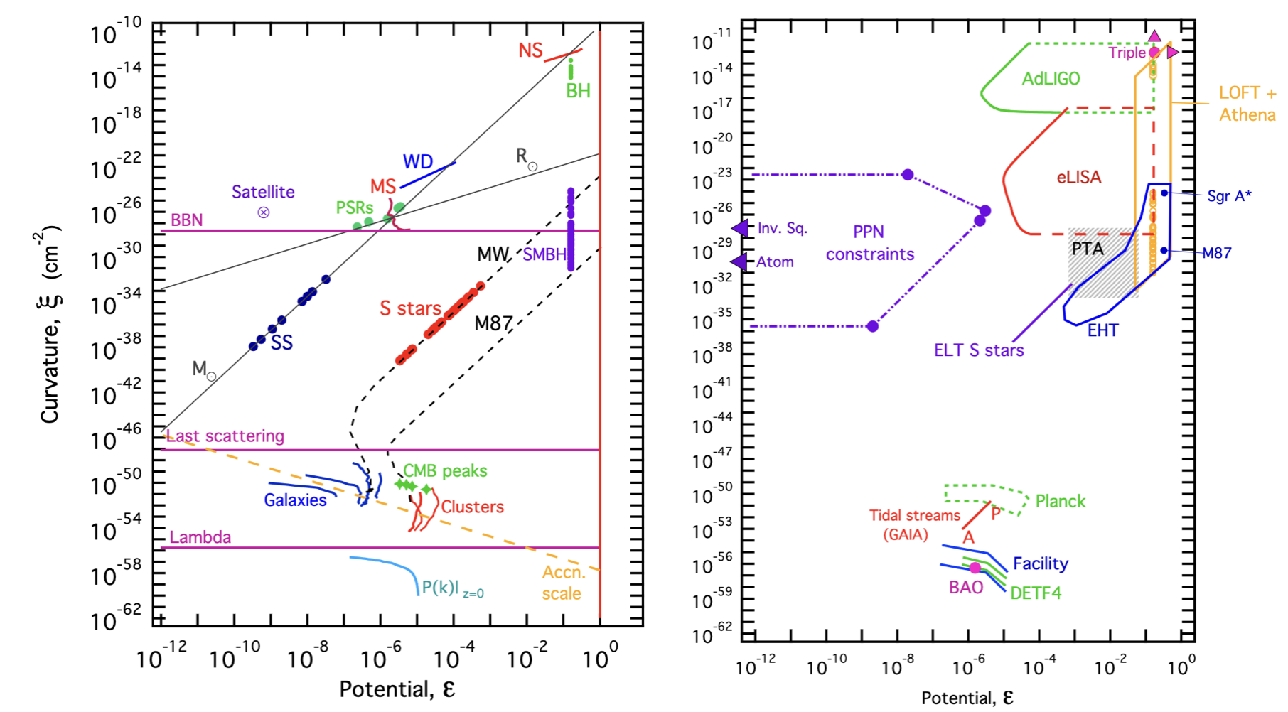
Figure 1: Physical phenomena and experimental constraints in the compactness ($\epsilon$) and curvature ($\xi$) plane. From Baker et al (2015). Abbreviations: SS = planets of the Solar System, MS = Main Sequence stars, WD = white dwarfs, PSRs = binary pulsars, NS = individual neutron stars, BH = stellar mass black holes, MW = the Milky Way, SMBH = supermassive black holes, BBN = Big Bang Nucleosynthesis.
On the other hand, it can be useful to distinguish different regimes of gravity. To take some commonly used terminologies in the literature:
- Weak fields regime: low energy tests of gravity, such as those performed in the solar system, for which the gravitational fields are weak and almost static.
- Strong fields regime: focusing on high density objects. These regimes are often quantified by the values of their compactness $\epsilon = GM/(c^2R)$ and curvature $\xi \propto GM/(R^3c^2)$, for an object of typical mass $M$ and characteristic length $R$ from that object (see Baker et al (2015)). Near the event horizon of a black-hole $\epsilon \sim 0.5$, for a neutron-star $\epsilon \sim 0.2$, while for solar system objects $\epsilon \sim 10^{-6}$ for the surface of the Sun to $\epsilon \sim 10^{-9}$ on Earth. As illustrated on Figure 1, strong gravity regimes are the ones of black holes and neutron stars.
- Dynamical gravity regime: exploring high velocity objects in which the gravitational field can vary strongly and quickly, such as orbiting neutron stars.
- Extreme gravity regime: where both high compactness and high velocities are involved, like mergers of black-holes and neutron stars.
- Quantum gravity regime: regime in which possible quantum effects of gravity are to be expected as near primordial or black hole singularities. Unfortunately, no experiment is yet able to distinctly probe such a regime, which would correspond to $\epsilon =1$ and $\xi\sim 10^{65}$, way out of Figure 1.
Most of the tests of general relativity to date are probing the weak field regime, the exception being gravitational waves and black hole physics. Of course, the distinction between all these regimes, and especially between dynamical, extreme and strong, is muddled most of the time, but it is useful to introduce them simply as helpers for our discussion. We refer to Yunes et al (2024), Baker et al (2015) as well as Will (2018), for a finer definition and discussion of these regimes. Unfortunately, one can argue that our incapacity to probe the quantum regime of gravity is one of the major hurdles today for fundamental physics at large. Specific detections, such as the signature of primordial gravitational waves coming from inflation with the measurement of primordial $B$-modes would be widely considered as major breakthrough in the exploration of these regimes.
The measurement of fundamental constants on various scales also provides a very powerful constraint on the nature of gravity, which we will leave for the next lecture. These measures are both local and astrophysical and in the weak and strong field regimes. Furthermore, we leave the discussion of cosmological constraints for their own dedicated lecture, such that this class focuses on local and astrophysical constraints.
Local validation of GR: lab and solar system weak fields tests of the EEP
Let us start with some local and high precision tests of the three building blocks of the EEP. All the tests discussed below are extremely precise and often based on high precision quantum measurements. They test only the validity of the EEP and hence whether gravity is described by a metric theory (see our previous lecture) and hence whether a curved space-time interpretation of gravity holds.
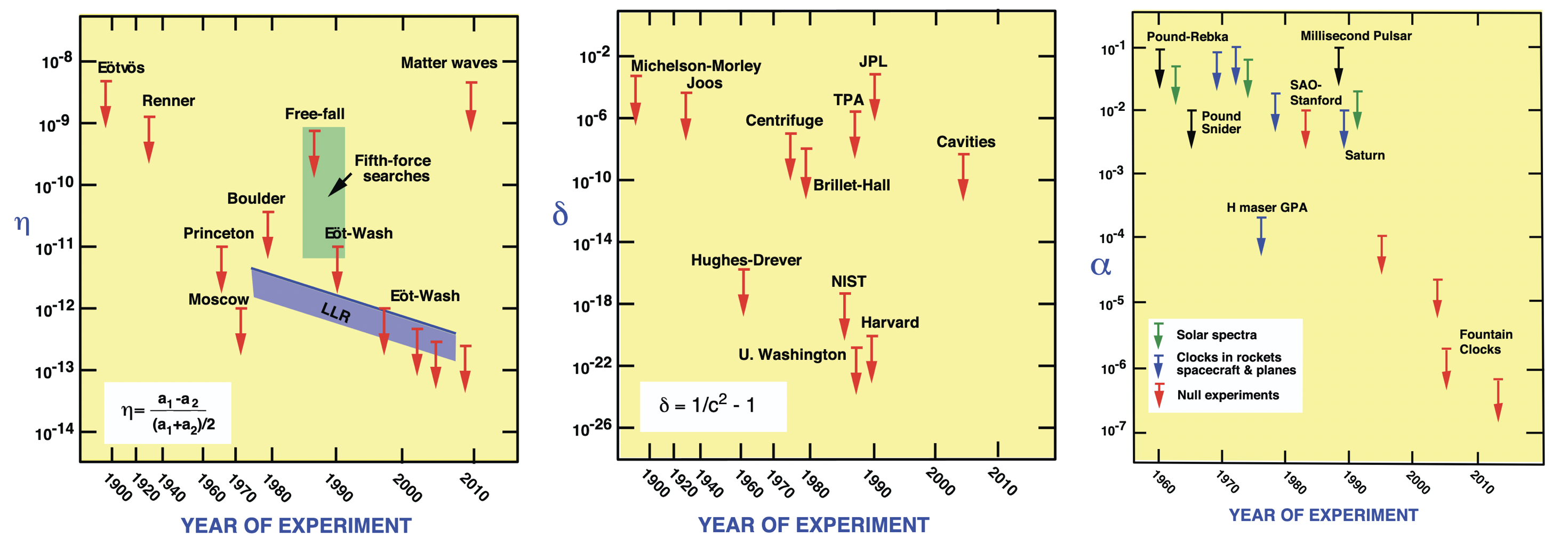
Figure 2: Some tests of the EEP. Left: tests of the WEP through measurement of $\eta$. Center: tests of the LLI through measurement of $\delta$. Right: tests of LPI through measurements of $\tilde{\alpha}$. Adapted from Will 2014.
Tests of the weak equivalence principle and free fall
The way to probe the UFF and hence quantify the validity of the WEP (and by extension the EEP) is to measure the quantity $\eta$, called the Eötvös parameter:
\[\boxed{ \eta = 2\frac{|\vec{a}_A - \vec{a}_B|}{|\vec{a}_A + \vec{a}_B|} }\]when considering two bodies $A$ and $B$ with different compositions and respective acceleration $\vec{a}_A$ and $\vec{a}_B$. Clearly, in the case of a perfect validity of the WEP one expects $\vec{a}_A = \vec{a}_B$ and thus $\eta =0$.
There are multiple ways to tests the EEP in the Solar system and beyond with a very high accuracy. The core idea is always to compare two bodies of different composition accelerating in the same gravitational field and seek for minute difference between their acceleration once all possible spurious effects (like drag) have been taken into account. The way to do so in practice consist of using tools such as torsion balances. The upper bounds of $\eta$ found by various experiments at different times can be found on the left panel of Figure 2.
The most competitive bound to date on $\eta$, is by far given by the MICROSCOPE experiment (Touboul et al (2022)). Using orbiting masses in free fall around the Earth inside a satellite experiment, the final results of the MICROSCOPE mission give a constraint on $\eta$ for a pair of titanium and platinum of
\[\begin{equation} \boxed{ \eta = (-1.5 \pm 2.7)\times 10^{-15}. } \end{equation}\]For more on MICROSCOPE results and their impact, see also the review of Bergé et al 2023.
Tests of the LLI and ether drift
Tests of the validity of the local Lorentz invariance can take multiple forms, but many of them consist of generalizations and refinement of the Michelson-Morley experiment, trying to use interferometry in order to detect possible changes in the value of the speed of light in different direction of motion. Possible variation of the speed of light $c$ in a direction compared to a reference value $c_0$ are quantified by the parameter:
\[\boxed{\delta = \left\vert 1-\frac{c^{-2}_0}{c^2} \right\vert}\]Different measurements of $\delta$ can be found in the middle panel of Figure 2. The best constraint to date on this value is
\[\boxed{\delta \lesssim 10^{-26},}\]obtained using so-called Hughes–Drever-type experiments Chupp 1989. These experiments do not focus on light propagation but instead seek for a possible dependence of a nucleus’s resonance frequency as the Earth carries it around. In order to reach such a precision, they exploit modern quantum technologies such as laser cooled trapped atoms and ions.
However, $\delta$ is an “old school” figure of merit for LLI violations. Today, possible violations of the Lorentz invariance are more finely measured using the so called standard model extension (SME) tables. These contain hundred of different coefficients quantifying all the possible violations of CPT and Lorentz symmetry. For a complete up to date table, see the review of Kostelecky and Russell (2026).
Tests of the LPI and gravitational redshift
General relativity, under the assumption of the perfect validity of the EEP is able to derive a precise a formula for the so-called gravitational redshift experienced by a photon moving in a gravitational field. Indeed, from the Newtonian limit derivation discussed in our previous lecture, it is possible to show that, considering two points at rest in a gravitational field and a photon emitted from on point at a frequency to another will $\nu_{em}$ will be received with another frequency $\nu_{ref}$ such as:
\[\boxed{\frac{\nu_{emm}- \nu_{rec}}{\nu_{rec}} = (1+\tilde{\alpha})\frac{\Delta \Phi}{c^2}}\]with $\tilde{\alpha}=0$ if LPI is valid.
Proof
We saw in the previous class that, within GR and in the Newtonian limit, $g_{00} = -\left(1 + \frac{2\Phi}{c^2}\right)$.
Consider an observer at rest at a fixed position in a static gravitational field, i.e. one whose metric does not depend on the time coordinate $t$. Setting $\mathrm{d}x^i = 0$ in $\mathrm{d}s^2 = g_{\mu\nu}\mathrm{d}x^\mu \mathrm{d}x^\nu = -c^2\mathrm{d}\tau^2$, the proper time measured by this observer is
\[\mathrm{d}\tau^2 = \left(1 + \frac{2\Phi}{c^2}\right)\mathrm{d}t^2 \qquad \Longrightarrow \qquad \mathrm{d}\tau \simeq \left(1 + \frac{\Phi}{c^2}\right)\mathrm{d}t ,\]where the last step is the first-order expansion in \(\Phi/c^2 \ll 1\). Here \(\mathrm{d}t\) is the coordinate time, a bookkeeping label shared by the whole spacetime, while $\mathrm{d}\tau$ is the proper time, the time actually measured by a physical clock sitting at that location. The two differ by the local value of the potential: clocks deeper in the potential well ($\Phi$ more negative) tick more slowly.
Let an emitter at rest at position \(\vec{x}_{\rm em}\) send out two successive crests of a light wave, and let a receiver at rest at $\vec{x}_{\rm rec}$ collect them. Because the metric is static, the spacetime geometry is identical at the moment of the first crest and at the moment of the second: the two crests therefore follow exactly the same trajectory and take exactly the same coordinate time to travel from emitter to receiver. Whatever that travel time is — and we never need to compute it — it cancels in the difference, so
\[\Delta t_{\rm rec} = \Delta t_{\rm em} \equiv \Delta t .\]The coordinate period of the signal is unchanged along the path. This is the whole content of the geometrical part of the effect, and it relies only on staticity.
Applying the relation between proper and coordinate time at each end,
\[\Delta \tau_{\rm em} \simeq \left(1 + \frac{\Phi_{\rm em}}{c^2}\right)\Delta t , \qquad \Delta \tau_{\rm rec} \simeq \left(1 + \frac{\Phi_{\rm rec}}{c^2}\right)\Delta t .\]A frequency is the inverse of a period measured by a local physical clock, $\nu = 1/\Delta\tau$. Hence
\[\frac{\nu_{\rm rec}}{\nu_{\rm em}} = \frac{\Delta\tau_{\rm em}}{\Delta\tau_{\rm rec}} = \frac{1 + \Phi_{\rm em}/c^2}{1 + \Phi_{\rm rec}/c^2} \simeq 1 - \frac{\Phi_{\rm rec} - \Phi_{\rm em}}{c^2} .\]Defining $\Delta\Phi \equiv \Phi_{\rm rec} - \Phi_{\rm em}$, this is
\[\frac{\nu_{\rm em} - \nu_{\rm rec}}{\nu_{\rm rec}} \simeq \frac{\Delta\Phi}{c^2} ,\]which is the standard gravitational redshift: light climbing out of a potential well ($\Delta\Phi > 0$) arrives with a lower frequency.
Notice what the derivation above never used: the nature of the clock. We never asked whether the emitter was a $^{57}$Fe nucleus, a caesium atom or a hydrogen maser. We implicitly assumed that a given atomic transition, measured locally in the freely falling frame of the emitter, always yields the same frequency $\nu^{(0)}$ — a universal constant of nature. This assumption is precisely local position invariance (LPI).
Suppose now that LPI is violated: the internal physics of the clock — through a possible dependence of the fundamental constants on the ambient gravitational potential — makes the locally measured transition frequency depend on where the clock sits,
\[\nu^{\rm local}(\Phi) = \nu^{(0)}\left(1 + \tilde{\alpha}\,\frac{\Phi}{c^2}\right) ,\]where $\tilde{\alpha}$ is a dimensionless parameter which may differ from one type of clock to another.
The measurement now involves two effects. Repeating Step 2 with $\nu_{\rm em} \to \nu^{\rm local}(\Phi_{\rm em})$, the signal arrives at the receiver with
\[\nu_{\rm rec} \simeq \nu^{(0)}\left(1 + \tilde{\alpha}\frac{\Phi_{\rm em}}{c^2}\right)\left(1 - \frac{\Delta\Phi}{c^2}\right) .\]But the receiver does not know $\nu^{(0)}$: it compares the incoming signal to its own identical clock, which ticks at $\nu^{(0)}\left(1 + \tilde{\alpha}\Phi_{\rm rec}/c^2\right)$. Taking the ratio and keeping first order,
\[\frac{\nu_{\rm rec}}{\nu_{\rm em}} \simeq \left(1 - \tilde{\alpha}\frac{\Delta\Phi}{c^2}\right)\left(1 - \frac{\Delta\Phi}{c^2}\right) \simeq 1 - (1 + \tilde{\alpha})\frac{\Delta\Phi}{c^2} ,\]which gives the announced result
\[\boxed{\frac{\nu_{\rm em} - \nu_{\rm rec}}{\nu_{\rm rec}} = (1 + \tilde{\alpha})\frac{\Delta\Phi}{c^2}} \qquad \Delta\Phi \equiv \Phi_{\rm rec} - \Phi_{\rm em} .\]Different measures on $\tilde{\alpha}$ are found in the right panel of Figure 2. The latest bound on this parameter comes from constraints comparing the rate of atomic clocks contained in the Galileo Satellites (GSATs), which were accidentally launched on elliptic orbits. These data allow to reach a constraint of
\[\boxed{\tilde{\alpha} = (-4.5 \pm 3.1) \times 10^{-5}}\]when taking the mean posterior of three different clocks Herrmann et al (2018). LPI is also tested by looking for possible space-time variations of the fundamental constants, which will be the topic of the next lecture.
EEP violations, formalisms and fifth force
As we briefly discussed above, the EEP has been tested independently over a wide range of length scales and physical regimes, and experimental efforts continue to improve these tests with ever-increasing precision. A variety of theoretical formalisms have been developed to parameterize possible violations beyond the traditional quantities $\eta$, $\delta$, and $\tilde{\alpha}$. Examples include the $TH\epsilon\mu$ and $c^{-2}$ formalisms, as well as the Standard-Model Extension (SME), which we discussed above. In parallel, numerous experiments have tested the gravitational inverse-square law at short distances in search of deviations from the Newtonian $r^{-2}$ prediction, motivated, for example, by scenarios involving extra compact spatial dimensions. A comprehensive discussion of these experiments is beyond the scope of this review, and we refer the reader to Will (2018) for an extensive overview of both the theoretical frameworks and the current experimental constraints of the EEP.
As a side note, we emphasize that even if a violation of the EEP were ever detected, its theoretical interpretation would be far from straightforward. Within the framework of General Relativity, such a result would clearly indicate the existence of physics beyond a purely metric theory of gravity, implying an additional interaction coupling to matter beyond geodesic motion in curved spacetime. For this reason, such a mechanism is also often referred to as a fifth force. To illustrate this point, consider a neutral ball and a charged ball falling in the presence of a magnetic field, assuming the existence of electromagnetism is unknown. One would infer a violation of the EEP because the two bodies would not follow the same trajectories and conclude that gravity is not pure geometry. However, the more appropriate interpretation would be the existence of an additional fundamental interaction rather than a breakdown of the equivalence principle itself. Ultimately, the physical significance of an observed EEP violation can only be established within a broader theoretical framework capable of explaining the underlying mechanism responsible for the deviation. However, the current data clearly impose the existence of such force to be either weak, or restrained on some specific scales (very small or very large).
Post-Newtonian parametrization: Astrophysical validation of GR and its dynamics
The previous discussion focused on the experimental validation of the EEP, and hence on whether or not gravity can be described by a metric theory (probing mostly the “S” type axioms). However, we did not yet constrain the dynamics of gravity (mostly D1).
In order to do so, it is common to introduce the so-called Parametrized Post-Newtonian (PPN) formalism, developed in its modern form Will and Nordtvedt (1972). This formalism provides ten measurable coefficients which quantify deviations from the dynamics of GR within any metric theory of gravity.
The idea is quite simple. The leading-order approximation of GR that we discussed in the first lecture is known as the Newtonian approximation. Pushing the expansion one order further in the small parameter $\epsilon$, one obtains the post-Newtonian approximation of General Relativity. In this framework, for a static, spherically symmetric source of mass $M$, the metric in isotropic coordinates reads:
\[\begin{align} &\boxed{g_{00}\simeq -1 + 2\frac{GM}{rc^2} - 2\left(\frac{GM}{rc^2}\right)^2} &\boxed{g_{jk}\simeq \left(1 + 2\frac{GM}{rc^2}\right)\delta_{jk}} \end{align}\]Post-Newtonian general relativity
The full derivation from the geodesic and Einstein equations is quite lengthy but follows the same steps as the Newtonian approximation.
A much quicker way to reach these terms is to assume the well-known exact Schwarzschild solution of Einstein equation for a spherically symmetric system:
Expanding in $U \equiv GM/(rc^2)$:
\[g_{00} = -\left(1 - 2U + 2U^2\right) + \mathcal{O}(U^3), \qquad g_{jk} = (1+2U)\,\delta_{jk} + \mathcal{O}(U^2),\]which are the boxed equations above.
Taking these terms into account leads to a correction to the Newtonian gravitational force, such that:
\[\vert \vec{F}_G \vert \simeq \frac{Gm_1m_2}{r^2}\left(1 + \frac{3\ell^2}{c^2 r^2}\right)\]with $\ell = r^2\dot\varphi$ the specific (i.e. per unit reduced mass) orbital angular momentum. From this expression, one can infer a precession of the orbit, with an advance of the perihelion per orbital period of
\[\frac{\Delta \varpi}{\Delta t} = \frac{6\pi GM}{c^2\,a(1-e^2)},\]where $a$ is the semi-major axis and $e$ the eccentricity of the orbit. Furthermore, the post-Newtonian terms also allow for the prediction of the deflection of a light ray grazing a massive source with impact parameter $b$:
\[\delta\theta = \frac{4GM}{c^2 b}\]These are among the most famous predictions of General Relativity. An anomalous perihelion advance of Mercury was known since Le Verrier (1859) (who estimated $\sim 38’’$ per century; the modern value is $\simeq 43’’$ per century), matching accurately the post-Newtonian prediction of GR. The light deflection was predicted to be $\sim 1.75’’$ at the Sun’s limb — twice the value obtained from a naive Newtonian corpuscular calculation (Soldner 1801), precisely because of the spatial part of the metric — and was confirmed by the Eddington–Dyson solar-eclipse expeditions of 29 May 1919. Together with gravitational redshift and the Shapiro effect, they are known as the “four classical tests of general relativity”.
Proof
1. Orbits of massive particles and the perihelion advance.
Consider a test particle in the equatorial plane $(\theta=\pi/2)$ of the Schwarzschild geometry. Staticity and spherical symmetry provide two conserved quantities along geodesics, the energy per unit mass $E = -g_{00}c^2\dot t$ and the angular momentum per unit mass $\ell = r^2\dot\varphi$ (dots denote derivatives with respect to proper time). Inserting these into $g_{\mu\nu}\dot x^\mu \dot x^\nu = -c^2$ and introducing $u \equiv 1/r$, one obtains the relativistic Binet equation
\[\frac{d^2u}{d\varphi^2} + u = \frac{GM}{\ell^2} + \frac{3GM}{c^2}u^2 .\]The first term on the right-hand side alone gives the Newtonian ellipse $u_0 = \frac{GM}{\ell^2}\left(1+e\cos\varphi\right)$; the second term is the $\mathcal{O}(\epsilon)$ relativistic correction (it is equivalent to the corrected force quoted in the main text). Treating it perturbatively, the resonant part of the source term ($\propto \cos\varphi$) produces a secular drift, and the solution takes the form
\[u \simeq \frac{GM}{\ell^2}\Big[1+e\cos\big((1-\delta)\varphi\big)\Big], \qquad \delta = \frac{3(GM)^2}{c^2\ell^2}.\]The orbit thus returns to perihelion after an angle $2\pi/(1-\delta) \simeq 2\pi(1+\delta)$, i.e. it precesses by $\Delta \varpi = 2\pi\delta$ per orbit. Using the Newtonian relation $\ell^2 = GMa(1-e^2)$,
\[\Delta \varpi = \frac{6\pi GM}{c^2 a(1-e^2)}.\]For Mercury ($a = 5.79\times 10^{10}\,\mathrm{m}$, $e=0.206$, period $88$ days), this gives $\Delta \varpi \simeq 0.103’’$ per orbit, i.e. $\simeq 43’’$ per century.
2. Deflection of light.
For a null geodesic, the same derivation with $g_{\mu\nu}\dot x^\mu\dot x^\nu = 0$ gives
\[\frac{d^2u}{d\varphi^2} + u = \frac{3GM}{c^2}u^2 .\]At zeroth order, the solution is a straight line with impact parameter $b$: $u_0 = \sin\varphi/b$. Writing $u = u_0+u_1$ and solving at first order,
\[u = \frac{\sin\varphi}{b} + \frac{GM}{2c^2b^2}\left(3+\cos 2\varphi\right).\]The incoming and outgoing asymptotes correspond to $u\to 0$, reached at $\varphi = -\epsilon_1$ and $\varphi = \pi + \epsilon_2$ with $\epsilon_{1,2} = 2GM/(c^2b)$. The total deflection is therefore
\[\delta\theta = \epsilon_1+\epsilon_2 = \frac{4GM}{c^2b}.\]Exactly half of this deflection comes from $g_{00}$ (the “Newtonian” part) and half from the spatial curvature encoded in $g_{jk}$ — which is why the PPN result below carries the factor $(1+\gamma)/2$.
The idea of the PPN formalism is to allow for possible deviations from the GR prediction through new parameters $\beta$, $\gamma$, as:
\[\begin{align} &\boxed{g_{00}\simeq -1 +2\frac{GM}{c^2r} - 2\beta\left(\frac{GM}{c^2r}\right)^2} &\boxed{g_{jk}\simeq \left(1 +2\gamma\frac{GM}{c^2r}\right)\delta_{jk}} \end{align}\]Each such parameter is introduced carefully so as to be physically meaningful. Performing the proper and full post-Newtonian expansion for a general fluid source, and assuming only that the theory is a metric theory, one ends up with the following ten parameters:
-
$\gamma$ — how much space curvature is produced by unit rest mass. It is the coefficient of the spatial part of the metric, $g_{ij} = \left(1+2\gamma\,GM/rc^2\right)\delta_{ij}$, and is therefore probed by relativistic particles: a photon feels $g_{00}$ and $g_{ij}$ equally, whereas a slow test mass feels only $g_{00}$ at Newtonian order. We will rediscuss how to measure $\gamma$ at the end of this section.
-
$\beta$ — how much nonlinearity there is in the superposition law of gravity (in Newtonian gravity, gravitational fields add linearly, not in general relativity, as “gravity gravitates”). This is encoded in the coefficient of the $\left(GM/rc^2\right)^2$ term in $g_{00}$. This is directly felt by massive particles in orbits. As for $\gamma$, we will rediscuss how to measure $\gamma$ at the end of this section.
-
$\xi$ — preferred-location effects: does local gravitational physics depend on where you are, i.e. on the ambient potential of the surrounding matter? Equivalently, $\xi \neq 0$ produces a Galaxy-induced anisotropy of the locally measured gravitational constant. It is sometimes called the Whitehead parameter, after the theory it was introduced to test. It is bounded in the Solar System by gravimeter searches for anomalous Earth tides, and far more tightly by observing the spin precession of solitary millisecond pulsars.
-
$\alpha_1, \alpha_2, \alpha_3$ — preferred-frame effects, i.e. a violation of local Lorentz invariance in the gravitational sector. They couple to the velocity $\vec{w}$ of the system with respect to the universal rest frame — operationally, the frame in which the CMB dipole vanishes. Observationally they appear as an orbital polarisation of binary pulsars ($\alpha_1$), a precession of the spin axis of the Sun or of solitary pulsars ($\alpha_2$), and a self-acceleration of spinning bodies along their spin axis ($\alpha_3$).
-
$\zeta_1, \zeta_2, \zeta_3, \zeta_4$, together with $\alpha_3$ — probe possible violations of the conservation of total momentum. ($\alpha_3$ plays a double role here: it tags both preferred-frame and non-conservative effects, which is why ten parameters answer only six physical questions.) A theory with $\alpha_3 = \zeta_i = 0$ is called semi-conservative; if in addition $\alpha_1 = \alpha_2 = 0$ it is fully conservative, and only $\gamma$ and $\beta$ survive — these two are the historical Eddington–Robertson–Schiff parameters, and the only ones probed by the three classical tests. Note finally that $\zeta_4$ is not an independent parameter: in any semi-conservative theory, $6\zeta_4 = 3\alpha_3 + 2\zeta_1 - 3\zeta_3$.
In General Relativity: $\gamma=\beta=1$ and $\xi=\alpha_i=\zeta_i=0$. Theories with $\alpha_3=\zeta_i=0$ are called semi-conservative, and fully conservative if in addition $\alpha_1=\alpha_2=0$. Every metric theory based on a Lagrangian is semi-conservative. Once a modified theory of gravity is considered, it is relevant to derive its predictions for the PPN parameters and confront them with experiments. We will come back to this for specific theories of modified gravity.
In terms of the PPN parameters, the predictions of a metric theory of gravity are, for the perihelion advance per orbit:
\[\boxed{\frac{\Delta \varpi}{\Delta t}= \frac{6\pi GM}{c^2a(1-e^2)}\cdot\frac{2+2\gamma-\beta}{3}}\]and for the deflection of light:
\[\boxed{\delta\theta = \left(\frac{1+\gamma}{2}\right)\frac{4GM}{c^2 b}}\]As such, any alternative theory of gravity wanting to compete with GR must predict values of the PPN parameters as compatible with experiments as those of GR.
Defining the PPN parameters
For a full discussion see chapter 4 of Will (2018). We simply copy here the key results of Will’s Box 4.1.
Consider a quasi-local Lorentz coordinate system in a specific (PPN) gauge. Let:
- $\rho$ = density of rest mass of a fluid element as measured in a local, freely falling, momentarily comoving frame.
- $u^\mu$ = four-velocity of the momentarily comoving frame, with $v^j \equiv u^j/u^0$ = coordinate velocity of the frame (and thus of the fluid element).
- $\rho^* = \rho u^0 \sqrt{-g}$ = “conserved” or baryonic mass density. Satisfies the exact continuity equation \(\rho^*_{,0} + \nabla \cdot (\rho^* \mathbf{v}) = 0\).
- $p$ = pressure as measured in a local, freely falling, momentarily comoving frame.
- $\Pi$ = internal energy per unit rest mass. It includes all forms of non-rest-mass, nongravitational energy, such as thermal energy, magnetic energy, etc.
- \(\mathbf{w}\) = coordinate velocity of the PPN coordinate system relative to the mean rest frame of the universe.
The full general expansion of the metric is:
\[\begin{aligned} g_{00} &= -1 + 2U + 2\left(\psi - \beta U^2\right) + \Phi^{\mathrm{PF}}, \\[4pt] g_{0j} &= -\left[2(1+\gamma) + \tfrac{1}{2}\alpha_1\right] V_j - \tfrac{1}{2}\left[1 + \alpha_2 - \zeta_1 + 2\xi\right] X_{,0j} + \Phi_j^{\mathrm{PF}}, \\[4pt] g_{jk} &= (1 + 2\gamma U)\,\delta_{jk}, \end{aligned}\]where
\[\begin{aligned} \psi ={}& \tfrac{1}{2}(2\gamma + 1 + \alpha_3 + \zeta_1 - 2\xi)\,\Phi_1 - (2\beta - 1 - \zeta_2 - \xi)\,\Phi_2 \\[2pt] &+ (1 + \zeta_3)\,\Phi_3 + (3\gamma + 3\zeta_4 - 2\xi)\,\Phi_4 - \tfrac{1}{2}(\zeta_1 - 2\xi)\,\Phi_6 - \xi\,\Phi_W . \end{aligned}\]Defining the potentials (primed quantities are evaluated at $\mathbf{x}’$, and commas denote partial derivatives, e.g. $X_{,0j}=\partial_t\partial_j X$ and $X_{jk} \equiv X_{,jk}$):
\[U = \int \frac{\rho'^{*}}{|\mathbf{x}-\mathbf{x}'|}\,d^3x', \qquad V_j = \int \frac{\rho'^{*} v'_j}{|\mathbf{x}-\mathbf{x}'|}\,d^3x', \qquad X = \int \rho'^{*}\,|\mathbf{x}-\mathbf{x}'|\,d^3x',\] \[\Phi_1 = \int \frac{\rho'^{*} v'^{2}}{|\mathbf{x}-\mathbf{x}'|}\,d^3x', \qquad \Phi_6 = \int \frac{\rho'^{*}\left[\mathbf{v}'\cdot(\mathbf{x}-\mathbf{x}')\right]^2}{|\mathbf{x}-\mathbf{x}'|^3}\,d^3x',\] \[\Phi_2 = \int \frac{\rho'^{*} U'}{|\mathbf{x}-\mathbf{x}'|}\,d^3x', \qquad \Phi_3 = \int \frac{\rho'^{*} \Pi'}{|\mathbf{x}-\mathbf{x}'|}\,d^3x', \qquad \Phi_4 = \int \frac{p'}{|\mathbf{x}-\mathbf{x}'|}\,d^3x',\] \[\Phi_W = \int \rho'^{*}\rho''^{*}\, \frac{(\mathbf{x}-\mathbf{x}')}{|\mathbf{x}-\mathbf{x}'|^3}\cdot \left[ \frac{(\mathbf{x}'-\mathbf{x}'')}{|\mathbf{x}-\mathbf{x}''|} - \frac{(\mathbf{x}-\mathbf{x}'')}{|\mathbf{x}'-\mathbf{x}''|} \right] d^3x'\,d^3x''.\]and the preferred-frame potential:
\[\begin{aligned} \Phi^{\mathrm{PF}} &= (\alpha_3 - \alpha_1)\,w^2 U + (2\alpha_3 - \alpha_1)\,w^j V_j + \alpha_2\,w^j w^k X_{jk}, \\[4pt] \Phi_j^{\mathrm{PF}} &= -\tfrac{1}{2}\alpha_1\,w_j U + \alpha_2\,w^k X_{jk}. \end{aligned}\]The latest experimental constraints on these parameters are gathered in the following table (entries without error bars are upper limits on the absolute value):
| Parameter | Best constraint | Effect | Source (year) |
|---|---|---|---|
| $\gamma-1$ | $(2.1 \pm 2.3) \times 10^{-5}$ | Shapiro time delay | Cassini — Bertotti et al. (2003) |
| $\beta-1$ | $(-1.6 \pm 1.8) \times 10^{-5}$ | Mercury perihelion + solar $J_2$ | MESSENGER — Genova et al. (2018) |
| $\xi$ | $3.9 \times 10^{-9}$ | Spin precession | Solitary millisecond pulsars — Shao & Wex (2013) |
| $\alpha_1$ | $-0.4^{+3.7}_{-3.1} \times 10^{-5}$ | Orbital polarization | PSR J1738+0333 — Shao & Wex (2012) |
| $\alpha_2$ | $1.6 \times 10^{-9}$ | Spin precession | Solitary millisecond pulsars — Shao et al. (2013) |
| $\alpha_3$ | $4 \times 10^{-20}$ | Self-acceleration | Pulsar spin-down statistics — Will (2014) |
| $\zeta_1$ | $0.02$ | Combined PPN bounds | Will (2014) |
| $\zeta_2$ | $1.3 \times 10^{-5}$ | Binary-pulsar self-acceleration ($\ddot\nu$, $\dddot\nu$) | Combined binary pulsars — Miao et al. (2020), improving Will (1992) |
| $\zeta_3$ | $1\times 10^{-8}$ | Newton’s 3rd law (lunar acceleration) | Bartlett & Van Buren (1986) |
| $\zeta_4$ | $0.006$ | Not independent: $6\zeta_4 = 3\alpha_3 + 2\zeta_1 - 3\zeta_3$ | Will (1976) |
| $\eta_N$ (SEP) | $(-6.6 \pm 7.2)\times 10^{-5}$ | Nordtvedt effect (Not independent, see below) | MESSENGER — Genova et al. (2018); LLR gives $(-0.2\pm 1.1)\times 10^{-4}$ — Hofmann & Müller (2018) |
Table 1: Latest constraints on the PPN parameters and the SEP. Updated version of the table of Will (2014), see also the version on wikipedia.
Some explanations on these measurements:
$\gamma$ can be measured by two observables, both carrying the same prefactor $(1+\gamma)/2$: the deflection of light, historically in Eddington’s 1919 eclipse expedition, and today through very-long-baseline interferometry (VLBI) of quasars and compact radio sources, which reaches $\vert\gamma-1\vert\lesssim 2\times 10^{-4}$ and the Shapiro time delay, i.e. the extra travel time of a signal passing near a massive body, which gives the tightest bound of all — the Cassini bound in Table 1. Note that this measurement was made in June 2002, during the spacecraft’s cruise phase, from the Doppler shift of a dual-band (X/Ka) radio link whose ray grazed the Sun at $1.6\,R_\odot$; Cassini only reached Saturn in 2004, orbiting it until 2017, exploring the physics of the giant planet and its moons. A complementary test exists on kiloparsec scales, combining strong gravitational lensing (which measures $\Phi+\Psi$) with stellar velocity dispersions (which measure $\Psi$ alone) in massive elliptical galaxies — e.g. the SLACS sample built from SDSS spectroscopy — currently constraining $\gamma$ at the few-percent level. A word of caution here: cosmological surveys such as DESI, Euclid and LSST do not measure the PPN $\gamma$. They constrain the gravitational slip $\eta \equiv \Phi/\Psi$ on Mpc scales, which is a logically distinct quantity (we will come back to this in the cosmology class). Screening mechanisms (chameleon, symmetron, Vainshtein discussed later) are designed precisely so that $\gamma\to1$ in the dense Solar-System environment while $\eta \neq 1$ survives cosmologically, so the two constraints are complementary rather than competing.
$\beta$ is never measured on its own, but always in combination with $\gamma$. For measurements of the perihelion advance of the inner planets, it is possible to constrain $(2+2\gamma-\beta)/3$. The best determination comes from radio tracking of MESSENGER in orbit around Mercury (2011–2015), and its accuracy is ultimately limited by the poorly known quadrupole moment of the sun’s gravitational field $J_2^\odot$, due to the flattening of its pole (oblateness) because of its rotation. Other measurements leading to $\beta$ are tests of the strong equivalence principle through measurements of the Nordtvedt effect, which we will discuss in the next section. In both cases $\beta$ is extracted only after injecting an independent value of $\gamma$ — in practice the Cassini bound, or simply $\gamma=1$, the two being equivalent at present precision.
Tests of the SEP: the Nordtvedt effect
While the EEP concerns test bodies, the Strong Equivalence Principle (SEP) extends the universality of free fall to bodies with non-negligible gravitational self-energy. In a metric theory violating the SEP, the gravitational (passive) mass $m_g$ and the inertial mass $m_i$ of a self-gravitating body differ by an amount proportional to its gravitational self-energy $E_g<0$:
\[\frac{m_g}{m_i} = 1 + \frac{\eta_N E_g}{mc^2}\]On the definition of $\eta_N$
For simplicity again, we set ourselves in a Newtonian context, but all of these equations can be properly derived in the Newtonian limit of General relativity.
Consider a large body like the moon or the earth. It has (negative binding) energy due to its self gravity \(E_g = -\int \frac{Gm(r)\rho(r)}{r}\text{d}r\). Importing the special relativistic fact that energy contributes to mass, we can say that its total inertial mass is \(m_i c^2 = m_0c^2 + E_g\), with $m_0$ the sum of the mass of all its constituent and their binding energies.
Now, if the strong equivalent principle (SEP) is true, \(m_gc^2 = m_ic^2 = m_0c^2 + E_g\) and hence “the gravitational energy also gravitates” and it does so identically for every body independently of its composition (generalisation of the WEP including gravitational energy).
If the SEP is violated, we might consider that only a fraction of \((1+\eta_N)E_g\) of the gravitational energy gravitates and thus enters \(m_g\), hence \(m_g c^2 = m_0c^2 + (1+\eta_N) E_g = m_ic^2 + \eta_N E_g\) and:
\[\frac{m_g}{m_i} = \frac{m_ic^2+\eta_N E_g}{m_i c^2} = 1 + \frac{\eta_N E_g}{m_ic^2}\]So $1+\eta_N$ really is the fraction of gravitational energy that does gravitate. Depending on the sign of $\eta_N$, gravitational energy gravitates less (\(\eta_N < 0\)) or more (\(\eta_N > 0\)) than it contributes to the inertial mass.
where $\eta_N$ is the Nordtvedt parameter ($\eta_N=0$ in GR). Since $E_g/mc^2 \simeq -4.6\times 10^{-10}$ for the Earth and $\simeq -1.9\times 10^{-11}$ for the Moon, a nonzero $\eta_N$ would make the Earth and the Moon fall differently towards the Sun, polarizing the lunar orbit in the direction of the Sun — the Nordtvedt effect (Nordtvedt 1968), which is precisely tracked by Lunar Laser Ranging (LLR).
Remarkably, $\eta_N$ is not a new parameter: within the PPN formalism it can be re-expressed as
\[\eta_N = 4\beta - \gamma - 3 - \frac{10}{3}\xi - \alpha_1 +\frac{2}{3}\alpha_2 - \frac{2}{3}\zeta_1 - \frac{1}{3}\zeta_2,\]which reduces to $\eta_N = 4\beta-\gamma-3$ for fully conservative theories. Tests of the SEP therefore constrain a combination of the PPN parameters (this is how the MESSENGER bound on $\beta$ in Table 1 is obtained, combining $\eta_N$ with the Cassini bound on $\gamma$). In a sense a difference of $\eta_N$ between two bodies of different masses lead to a differential acceleration just like a violation of the WEP measured by the Eötvös parameter $\eta$.
Another related probe of the SEP is the constancy of the gravitational constant $G$, which will be discussed in the next lecture.
Compact objects: the strong-field and dynamical regimes of gravity
All the tests discussed so far were in the weak-field regime, i.e. they involve bodies with negligible compactness ($\epsilon \lesssim 10^{-6}$). Neutron stars change this: with $M\simeq 1.4\,M_\odot$ packed into $R\simeq 10$ km, they reach $\epsilon \simeq 0.2$, only a factor of a few below a black hole ($\epsilon = 0.5$ at the horizon). We thus enter the strong-field regime of gravitational tests. When such an object is a pulsar — a magnetised neutron star whose beamed radio emission sweeps past us once per rotation — it becomes a clock of extraordinary stability, and its orbital motion can be tracked with a precision no Solar-System experiment can match. All objects with high compactness are known as compact objects. The most extreme of them are black holes, which we now know exist without any doubt. While GR predicts their existence, alternative theories of gravity may predict differences in their structure and behavior.
Furthermore, binaries of compact objects orbit each other at highly relativistic speeds: the pulsar B1913+16 has an orbital velocity of a few hundred km/s, i.e. $v/c\sim 10^{-3}$, and merging binaries reach $v/c\sim 0.5$. Compact binaries therefore also probe the dynamical regime of gravity, inaccessible in the Solar System: such systems emit gravitational radiation, which can be studied either indirectly, through the energy loss of the binary, or now directly, through the detection of gravitational waves. Gravitational waves can be scrutinized in three complementary ways: their generation, their propagation and their polarization.
Alternative theories of gravity may predict significant deviations in these regimes — in the internal structure, the orbital dynamics or the gravitational radiation of compact objects. The PPN formalism, built on a weak-field expansion, is no longer the appropriate tool. Its role is played by new frameworks: the post-Keplerian (PK) formalism for binary pulsars, and modified Einstein–Infeld–Hoffmann (EIH) equations of motion, in which each strongly self-gravitating body carries “sensitivities” quantifying how its internal structure responds to the extra fields of the theory. We discuss briefly in the following sections how strong constraints, so far always in favour of GR, are extracted from compact objects.
Compact binaries
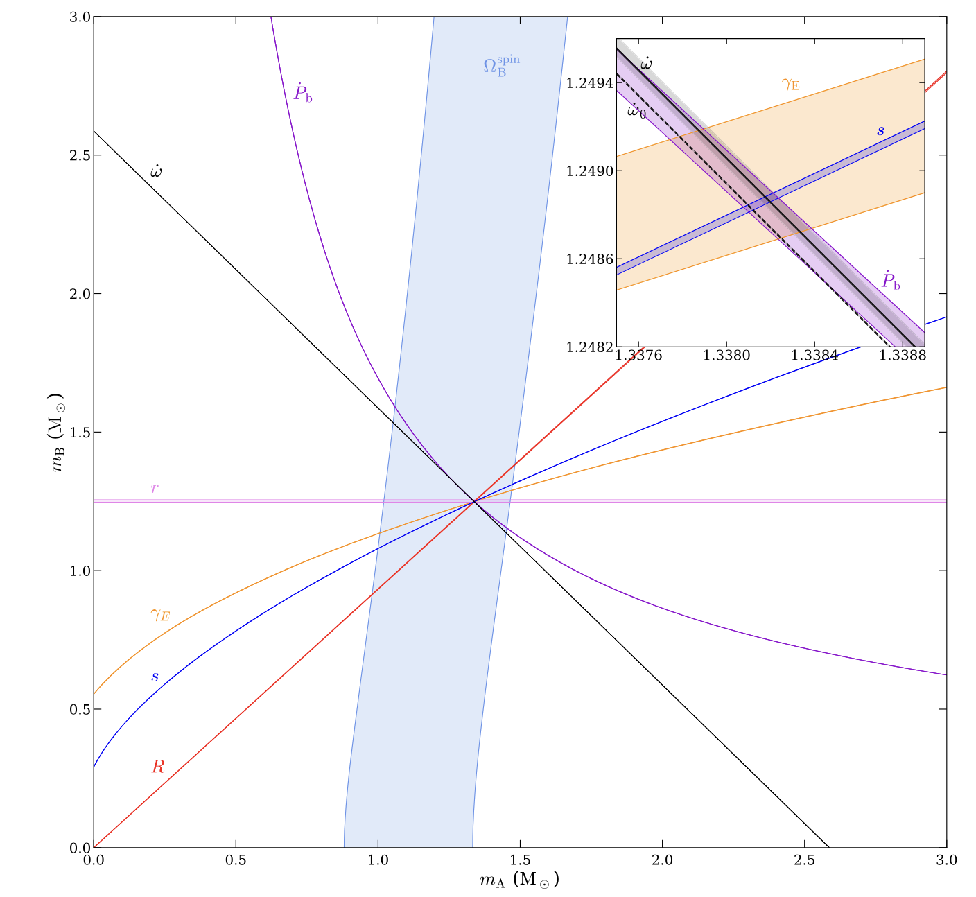
Figure 3: Mass-mass diagramm for the binary pulsar J0737−3039A/B. The $x$ and $y$ axis are the possible mass of the two pulsars. The lines represent the measurements of six Post-Keplerian parameters for this system, with the thikness being the error-bar. All lines cross at single point, in agreement with GR. From Kramer et al. 2021.
Timing a binary pulsar means fitting a model to the arrival times of its pulses over years. Five Keplerian parameters (orbital period $P_b$, eccentricity $e$, projected semi-major axis, longitude and time of periastron) describe the Newtonian orbit. Relativistic effects are then encoded in a set of theory-agnostic post-Keplerian parameters (Damour & Taylor 1992), the most important being:
- $\dot\omega$: the periastron advance (the pulsar analogue of Mercury’s perihelion shift, but reaching degrees per year);
- $\gamma_E$: the Einstein delay, combining second-order Doppler effect and gravitational redshift over the eccentric orbit;
- $\dot P_b$: the secular decay of the orbital period due to gravitational-wave emission;
- $r$ and $s$: the range and shape of the Shapiro delay of pulses grazing the companion.
In any given theory of gravity, each PK parameter is a definite function of the two (a priori unknown) masses $m_A$, $m_B$ only. Measuring two PK parameters therefore fixes the masses; every additional PK parameter is a test of the theory. This is elegantly visualized in the mass–mass diagram: each measured PK parameter draws a curve in the $(m_A,m_B)$ plane, and all curves must intersect in a single point if the theory is correct (see Figure 3).
Post-Keplerian parameters in GR
For a binary of masses $m_A$, $m_B$, total mass $M=m_A+m_B$, GR predicts (Damour & Deruelle 1986):
\[\dot\omega = \frac{3}{1-e^2}\left(\frac{P_b}{2\pi}\right)^{-5/3}\left(\frac{GM}{c^3}\right)^{2/3},\] \[\gamma_E = e\left(\frac{P_b}{2\pi}\right)^{1/3}\left(\frac{G}{c^3}\right)^{2/3}\frac{m_B(m_A+2m_B)}{M^{4/3}},\] \[\dot P_b = -\frac{192\pi}{5}\left(\frac{P_b}{2\pi}\right)^{-5/3}\left(\frac{G}{c^3}\right)^{5/3}\frac{m_Am_B}{M^{1/3}}\,\frac{1+\frac{73}{24}e^2+\frac{37}{96}e^4}{(1-e^2)^{7/2}},\]the last being the orbit-averaged energy loss from the quadrupole formula (Peters 1964). One can check that $\dot\omega$ reduces to the perihelion-advance formula of the previous section divided by $P_b$.
Two systems stand out. The pulsar B1913+16 (discovered 1974), also known as the Hulse–Taylor pulsar, provided the first evidence that gravitational waves exist: its measured orbital decay matches the GR quadrupole prediction, with $\dot P_b^{\rm obs}/\dot P_b^{\rm GR} = 0.9983 \pm 0.0016$ (Weisberg & Huang 2016) — the 1993 Nobel Prize. The double pulsar J0737−3039A/B, where both neutron stars were seen as pulsars, now provides the most precise strong-field test: seven PK parameters measured, with the predictions of GR regarding predictions on $\dot{P}_b$ verified at the $1.3\times 10^{-4}$ level (Kramer et al. 2021).
Beyond GR, the key new phenomenon is dipolar radiation. Theories with additional fields (e.g. scalar–tensor theories) generically predict gravitational radiation at $-1$PN order relative to the quadrupole, with amplitude $\propto (s_A-s_B)^2$, the difference of the sensitivities of the two bodies. It is thus best constrained by asymmetric systems: pulsar–white dwarf binaries such as PSR J1738+0333 rule out large regions of scalar–tensor parameter space (including “spontaneous scalarization”). Finally, the pulsar in the triple system J0337+1715, free-falling with its inner white-dwarf companion in the field of an outer white dwarf, provides the strong-field version of the Nordtvedt test: $\vert \Delta\vert = \vert \frac{m_g}{m_i}-1\vert \lesssim 2\times 10^{-6}$ (Voisin et al. 2020).
Pulsar timing arrays
A pulsar timing array (PTA) turns an ensemble of millisecond pulsars, timed over decades, into a Galaxy-sized gravitational-wave detector sensitive to the nanohertz band (periods of years). A passing gravitational-wave background perturbs the arrival times of all pulsars in a correlated way: in GR, the correlation between two pulsars depends only on their angular separation, following the Hellings–Downs curve (Hellings & Downs 1983), a quadrupolar signature specific to tensor modes. In 2023, the NANOGrav, EPTA+InPTA, PPTA and CPTA collaborations reported evidence for such a background with Hellings–Downs correlations, most plausibly from the population of supermassive black-hole binaries. As a gravity test, the shape of the correlation curve is itself the observable: extra scalar or vector polarizations, or a graviton mass, would deform it.
Gravitational waves: direct detections
Since GW150914 (September 2015), the LIGO–Virgo–KAGRA (LVK) network has detected on the order of a hundred compact-binary coalescences, including the binary neutron-star merger GW170817 with its electromagnetic counterparts. Each detection tests gravity in the strong-field and radiative regime simultaneously, along three axes.
1. Generation: the waveform
A coalescence waveform has three stages: the inspiral, described analytically by the post-Newtonian expansion (the same $\epsilon$-expansion as before, now pushed to high orders in $v/c$); the merger, requiring numerical relativity; and the ringdown, where the remnant black hole settles down by emitting quasi-normal modes (QNMs). At leading order the inspiral phase evolution depends on a single combination of the masses, the chirp mass $\mathcal{M} = (m_Am_B)^{3/5}/M^{1/5}$, via $\dot f = \frac{96}{5}\pi^{8/3}(G\mathcal{M}/c^3)^{5/3}f^{11/3}$.
Waveform tests come in three types, in close analogy with the PPN philosophy: (i) parametrized tests, where each PN coefficient of the phase is allowed to deviate fractionally from its GR value and the data constrain the deviations; (ii) inspiral–merger–ringdown consistency, comparing the remnant mass and spin inferred independently from the early and late waveform; (iii) black-hole spectroscopy: in GR the QNM frequencies and damping times are fixed uniquely by the remnant’s mass and spin (no-hair theorem), so measuring two modes overconstrains the system. All are so far consistent with GR (LVK, tests of GR with GWTC-3).
2. Propagation
Take the weak-field limit of the Einstein equations, $g_{\mu\nu} \simeq \eta_{\mu\nu} + h_{\mu\nu}$ with $\vert h_{\mu\nu}\vert \ll 1$, on a flat, non-expanding background. In vacuum, each Fourier mode of the transverse-traceless perturbation obeys
\[\boxed{\;\ddot{h}_{ij} + c^2 k^2\, h_{ij} = 0\;}\]where $k$ is the wavenumber and a dot denotes $\partial/\partial t$. This is the equation of a free harmonic oscillator of frequency $\omega = ck$: the wave propagates at exactly $c$, with no dispersion and no loss of amplitude.
Proof
Write $g_{\mu\nu} = \eta_{\mu\nu} + h_{\mu\nu}$ and keep only terms linear in $h$. We will follow the same reasoning as we did for the Newtonian limit without imposing the static limit. We will go quickly on the first part, as this computation is standard and can be found in most GR textbooks cited in our first class.
With the weak field limit, the Christoffel symbols become:
\[\Gamma^{(1)\rho}{}_{\mu\nu} = \tfrac12\big(\partial_\mu h^{\rho}{}_{\nu} + \partial_\nu h^{\rho}{}_{\mu} - \partial^{\rho} h_{\mu\nu}\big)\]Here and in everything that follows, we add an upper index $(1)$ to mean that we are computing the GR quantity at first order in the perturbation $h$.
For the Riemann tensor, only the derivative terms survive the first order approximation:
\[R^{(1)\rho}{}_{\sigma\mu\nu} = \tfrac12\big(\partial_\mu\partial_\sigma h^{\rho}{}_{\nu} - \partial_\mu\partial^{\rho}h_{\nu\sigma} - \partial_\nu\partial_\sigma h^{\rho}{}_{\mu} + \partial_\nu\partial^{\rho}h_{\mu\sigma}\big).\]From which we can compute the Ricci tensor, Ricci scalar and Einstein tensor:
\[R^{(1)}_{\sigma\nu} = R^{(1)\rho}{}_{\sigma\rho\nu} = \tfrac12\big(\partial_\rho\partial_\sigma h^{\rho}{}_{\nu} - \partial_\rho\partial^{\rho} h_{\nu\sigma} - \partial_\nu\partial_\sigma h^{\rho}{}_{\rho} + \partial_\nu\partial^{\rho}h_{\rho\sigma}\big),\]i.e., renaming $\sigma\to\mu$, $\rho\to\alpha$ and using the notations \(\Box = \partial_\alpha\partial^\alpha\) and \(h= h^{\rho}{}_{\rho}\):
\[R^{(1)}_{\mu\nu} = \tfrac12\big(\partial_\alpha\partial_\mu h^{\alpha}{}_{\nu} + \partial_\alpha\partial_\nu h^{\alpha}{}_{\mu} - \Box h_{\mu\nu} - \partial_\mu\partial_\nu h\big)\]and then:
\[R = g^{\mu\nu}R_{\mu\nu} = (\eta^{\mu\nu} - h^{\mu\nu})(R^{(0)}_{\mu\nu} + R^{(1)}_{\mu\nu})\]The zeroth-order Ricci tensor vanishes ($\eta$ is flat: $R^{(0)}_{\mu\nu}=0$), so at first order \(R^{(1)} = \eta^{\mu\nu}R^{(1)}_{\mu\nu}\):
\[R^{(1)} = \tfrac12\big(\partial_\alpha\partial_\mu h^{\alpha\mu} + \partial_\alpha\partial_\nu h^{\alpha\nu} - \Box h - \Box h\big)\]that is:
\[R^{(1)} = \partial_\mu\partial_\nu h^{\mu\nu} - \Box h\;\]and:
\[\;G^{(1)}_{\mu\nu} = \tfrac12\Big(\partial_\alpha\partial_\mu h^{\alpha}{}_{\nu} + \partial_\alpha\partial_\nu h^{\alpha}{}_{\mu} - \Box h_{\mu\nu} - \partial_\mu\partial_\nu h - \eta_{\mu\nu}\,\partial_\alpha\partial_\beta h^{\alpha\beta} + \eta_{\mu\nu}\,\Box h\Big)\;\]The linearized Einstein equations are therefore
\[\boxed{\tfrac12\Big(\partial_\alpha\partial_\mu h^{\alpha}{}_{\nu} + \partial_\alpha\partial_\nu h^{\alpha}{}_{\mu} - \Box h_{\mu\nu} - \partial_\mu\partial_\nu h - \eta_{\mu\nu}\,\partial_\alpha\partial_\beta h^{\alpha\beta} + \eta_{\mu\nu}\,\Box h\Big) = 8\pi G\, T_{\mu\nu},}\]a set of $10$ coupled linear second-order PDEs for the $10$ components $h_{\mu\nu}$. We will be able to reduce this number of degrees of freedom using the so-called gauge freedom.
We first introduce the trace-reversed perturbation:
\[\;\bar h_{\mu\nu} \equiv h_{\mu\nu} - \tfrac12 \eta_{\mu\nu}\, h\;\]Take the trace with $\eta^{\mu\nu}$, using $\eta^{\mu\nu}\eta_{\mu\nu} = \delta^\mu{}_\mu = 4$:
\[\bar h \equiv \eta^{\mu\nu}\bar h_{\mu\nu} = h - \tfrac12 \cdot 4 \cdot h = -h.\]The trace flips sign — hence the name. The map is an involution, so it inverts trivially:
\[h_{\mu\nu} = \bar h_{\mu\nu} - \tfrac12\eta_{\mu\nu}\bar h.\]Insert $h_{\mu\nu} = \bar h_{\mu\nu} - \tfrac12\eta_{\mu\nu}\bar h$ and $h = -\bar h$ into $G^{(1)}_{\mu\nu}$, term by term:
| term in $2G^{(1)}_{\mu\nu}$ | becomes |
|---|---|
| $\partial^\alpha\partial_\mu h_{\alpha\nu}$ | $\partial^\alpha\partial_\mu \bar h_{\alpha\nu} - \tfrac12\partial_\mu\partial_\nu \bar h$ |
| $\partial^\alpha\partial_\nu h_{\alpha\mu}$ | $\partial^\alpha\partial_\nu \bar h_{\alpha\mu} - \tfrac12\partial_\mu\partial_\nu \bar h$ |
| $-\Box h_{\mu\nu}$ | $-\Box \bar h_{\mu\nu} + \tfrac12\eta_{\mu\nu}\Box\bar h$ |
| $-\partial_\mu\partial_\nu h$ | $+\partial_\mu\partial_\nu\bar h$ |
| $-\eta_{\mu\nu}\partial_\alpha\partial_\beta h^{\alpha\beta}$ | $-\eta_{\mu\nu}\partial_\alpha\partial_\beta \bar h^{\alpha\beta} + \tfrac12\eta_{\mu\nu}\Box\bar h$ |
| $+\eta_{\mu\nu}\Box h$ | $-\eta_{\mu\nu}\Box\bar h$ |
The $\partial_\mu\partial_\nu\bar h$ coefficients sum to $-\tfrac12-\tfrac12+1 = 0$, and the $\eta_{\mu\nu}\Box\bar h$ coefficients to $\tfrac12+\tfrac12-1 = 0$. Both trace terms cancel identically. What survives:
\[\boxed{\;G^{(1)}_{\mu\nu} = -\tfrac12\Big(\Box \bar h_{\mu\nu} + \eta_{\mu\nu}\,\partial^\alpha\partial^\beta \bar h_{\alpha\beta} - \partial^\alpha\partial_\mu \bar h_{\alpha\nu} - \partial^\alpha\partial_\nu \bar h_{\alpha\mu}\Big)\;}\]Now, the split $g_{\mu\nu} = \eta_{\mu\nu} + h_{\mu\nu}$ is not unique and depends on a choice of an inertial frame in which it is evaluated. Consider the coordinate transformation that leaves the perturbations small:
\[x^\mu \;\longrightarrow\; x'^{\mu} = x^\mu + \xi^\mu(x), \qquad |\partial_\nu \xi^\mu| \ll 1.\]Transforming the metric tensor, \(g'_{\mu\nu} = \dfrac{\partial x^\alpha}{\partial x'^\mu}\dfrac{\partial x^\beta}{\partial x'^\nu} g_{\alpha\beta}\), with \(\dfrac{\partial x^\alpha}{\partial x'^\mu} = \delta^\alpha{}_\mu - \partial_\mu \xi^\alpha + \mathcal{O}(\xi^2)\), and keeping only first order in the small quantities $h$ and $\xi$:
\[g'_{\mu\nu} = \eta_{\mu\nu} + h_{\mu\nu} - \partial_\mu\xi_\nu - \partial_\nu\xi_\mu.\]The background $\eta_{\mu\nu}$ is unchanged, so the whole effect is absorbed into the perturbation:
\[\boxed{\;h_{\mu\nu} \;\longrightarrow\; h'_{\mu\nu} = h_{\mu\nu} - \partial_\mu\xi_\nu - \partial_\nu\xi_\mu \;=\; h_{\mu\nu} - (\mathcal{L}_\xi \eta)_{\mu\nu}\;}\]with $\xi_\mu \equiv \eta_{\mu\nu}\xi^\nu$ and where we introduced the Lie derivative \(\mathcal{L}_\xi T_{\mu\nu}\) which will be discussed and explained in a later lecture. This is a gauge transformation: $h_{\mu\nu}$ and $h’_{\mu\nu}$ describe the same physical spacetime.
This is formally identical to electromagnetism, $A_\mu \to A_\mu - \partial_\mu \lambda$, with the vector gauge parameter $\xi^\mu$ (4 functions) replacing the scalar $\lambda$. Linearized gravity is a gauge theory of a massless spin-2 field on flat space as we will discuss in a later lecture.
Now, from the expression of the Riemann tensor, we can compute easily that:
\[\;R^{(1)}_{\mu\nu\rho\sigma} = \tfrac12\big(\partial_\rho\partial_\nu h_{\mu\sigma} + \partial_\sigma\partial_\mu h_{\nu\rho} - \partial_\rho\partial_\mu h_{\nu\sigma} - \partial_\sigma\partial_\nu h_{\mu\rho}\big)\;\]Insert \(\delta h_{\mu\nu} = -\partial_\mu\xi_\nu - \partial_\nu\xi_\mu\) into $R^{(1)}_{\mu\nu\rho\sigma}$. Each of the four terms produces third derivatives of $\xi$ that pair off and cancel because partial derivatives commute:
\[\delta_\xi R^{(1)}_{\mu\nu\rho\sigma} = 0.\]So curvature — and hence tidal forces, geodesic deviation, everything observable — is gauge independent. Consequently $R^{(1)}{\mu\nu}$, $R^{(1)}$ and $G^{(1)}{\mu\nu}$ are gauge invariant too.
Apply the gauge transformation to the trace-reversed field. Using $\delta h = -2\partial_\alpha\xi^\alpha$:
\[\bar h'_{\mu\nu} = \bar h_{\mu\nu} - \partial_\mu \xi_\nu - \partial_\nu \xi_\mu + \eta_{\mu\nu}\,\partial_\alpha \xi^\alpha.\]Take the divergence:
\[\partial^\nu \bar h'_{\mu\nu} = \partial^\nu\bar h_{\mu\nu} - \underbrace{\partial^\nu\partial_\mu\xi_\nu}_{=\,\partial_\mu\partial_\alpha\xi^\alpha} - \Box\xi_\mu + \underbrace{\partial_\mu\partial_\alpha\xi^\alpha}_{\text{from }\eta_{\mu\nu}\text{ term}} = \partial^\nu\bar h_{\mu\nu} - \Box\xi_\mu.\]The two $\partial_\mu\partial_\alpha\xi^\alpha$ terms cancel, and we are left with a clean, decoupled transformation law. Recall that we are free to chose any $\xi^\mu$ we want without changing the physical conditions. So: we choose $\xi^\mu$ solving the inhomogeneous wave equation:
\[\Box\, \xi_\mu = \partial^\nu \bar h_{\mu\nu}=0\]this is known as imposing the Lorenz gauge:
\[\boxed{\partial^\nu \bar h_{\mu\nu} = 0}\]which are four conditions, one per value of $\mu$. Equivalently \(\partial^\nu h_{\mu\nu} = \tfrac12\partial_\mu h\), or \(g^{\mu\nu}\Gamma^{(1)\rho}{}_{\mu\nu}=0\) at linear order. The gauge is not yet fully fixed by this condition: any further coordinate transformation $\zeta^\mu$ with $\Box\zeta^\mu = 0$ preserves the condition. These $4$ residual functions can further be fixed by the transverse–traceless gauge in vacuum later.
Impose now the Lorenz gauge $\partial^\nu\bar h_{\mu\nu} = 0$ in Einstein equation. The last three terms vanish, leaving \(G^{(1)}_{\mu\nu} = -\tfrac12 \Box \bar h_{\mu\nu}\). Setting \(G^{(1)}_{\mu\nu} = 8\pi G\, T_{\mu\nu}\):
\[\;\Box\, \bar h_{\mu\nu} \;=\; -16\pi G\, T_{\mu\nu}, \qquad \partial^\nu \bar h_{\mu\nu} = 0\;\]with \(\Box = -\partial_t^2 + \nabla^2\), \(\ \bar h_{\mu\nu} = h_{\mu\nu} - \tfrac12\eta_{\mu\nu}h\).
Written directly in $h_{\mu\nu}$, using $h_{\mu\nu}=\bar h_{\mu\nu}-\tfrac12\eta_{\mu\nu}\bar h$ and $\bar h = -h$:
\[\Box\, h_{\mu\nu} = -16\pi G\Big(T_{\mu\nu} - \tfrac12 \eta_{\mu\nu} \mathcal{T}\Big), \qquad \mathcal{T} \equiv \eta^{\mu\nu}T_{\mu\nu}.\]We had $10$ components in $h_{\mu\nu}$, minus $4$ that can be fixed by the gauge functions $\xi^\mu$, minus $4$ residual conditions that will be discussed later, hence $2$ remaining physical propagating degrees of freedom — the two polarizations of a gravitational wave. This is a set of ten decoupled flat-space wave equations, each with a source.
Now, for the propagation of gravitational waves, we consider the vacuum \(T_{\mu\nu}=0\) and the wave equation becomes simply \(\Box h_{\mu\nu}=0\). Now, we remember that, even after fixing the Lorenz gauge, we still have an extra gauge freedom if we change coordinates as $x \to x^\mu + \zeta^\mu$ with $\Box \zeta^\mu=0$. In practice, one an choose to further impose the four conditions: $h=0$ and $h_{i0}=0$. This is called the traceless-transverse (TT) gauge. Combining Lorenz and TT gauges, we can deduce that $h_{00}=0$, such that the wave equation reduces to:
\[\Box h_{ij}=0\]Let’s now fourier transform in space. Writing $h_{ij}(t,\mathbf{x}) = h_{ij}(t,\mathbf{k})\,e^{i\mathbf{k}\cdot\mathbf{x}}$ turns $\partial_i^2 \to (i)^2k^2 = -k^2$, so $\Box h_{ij}=0$ becomes
\[-\frac{1}{c^2}\ddot{h}_{ij} - k^2 h_{ij} = 0 \qquad\Longleftrightarrow\qquad \ddot{h}_{ij} + c^2 k^2 h_{ij} = 0 .\]This equation holds for nearby sources, where the expansion of the Universe can be ignored. On cosmological distances the background is FLRW rather than Minkowski, and the equation acquires a friction term,
\[\ddot{h}_{ij} + 3H\dot{h}_{ij} + \frac{c^2k^2}{a^2}h_{ij} = 0 ,\]with $H = \dot a/a$ the Hubble rate and $k$ now a comoving wavenumber. On this point, see our cosmology lecture.
Now, we can look for the most general generalisation of this wave equation, inspired by the classical physics of waves. For each Fourier mode, the most general linear, second-order, homogeneous equation for $h_{ij}$ is
\[\boxed{\;\ddot{h}_{ij} \;+\; \nu_T\,\dot{h}_{ij} \;+\; \omega^2(k)\,h_{ij} \;=\; S_{ij}\;}\]where $\nu_T$ is a possible damping (lowering of the amplitude when propagating), $S_{ij}$ is a possible source and the dispersion relation, at first order, is
\[\omega^2(k) = c_T^2 k^2 + M_g^2 .\]Here $c_T$ is the tensor (gravitational-wave) propagation speed, which need not equal the speed of light $c$. \(M_g\) can be interpreted as a graviton mass. Getting back the correct units in order to get a mass, one finds \(\frac{M_g^2 c^4}{\hbar^2}\) where $M_g$ is the proper graviton mass. While this might seems a bit obscure now, we will discuss in the massive gravity lecture what “mass of the graviton” means exactly. $\nu_T$ is a damping rate (change of amplitude through the propagation of the wave). In a flat, static spacetime $\nu_T$ is forced to vanish by time-translation invariance: an oscillator in an unchanging background cannot lose energy to that rigid background. (A non-zero $\nu_T$ therefore requires an evolving background, which is why damping is the one entry in the table that is irreducibly cosmological). $S_{ij}$ collects any possible coupling to other tensor fields that might source the waves.
All these parameters have been constraints by the direct detection of gravitational waves:
-
Speed ($c_T$). The coincidence of GW170817 with the gamma-ray burst GRB 170817A, after a $40\;$Mpc journey, constrains \(-3\times10^{-15} < \frac{c_{\rm gw}}{c} - 1 < 7\times10^{-16}\) (Abbott et al. 2017). The tightness comes from the enormous lever arm: a fractional speed difference $\delta$ accumulates a delay $\sim \delta \times (40\;{\rm Mpc}/c) \approx \delta \times 4\times10^{15}\,$s, and the observed delay was $1.7\,$s. This single measurement eliminated entire classes of modified-gravity dark-energy models predicting $c_{\rm gw} \neq c$.
- Dispersion / mass ($M_g$). A graviton mass makes the group velocity frequency-dependent, \(\frac{v_g}{c} = \sqrt{1 - \frac{M_g^2c^4}{(\hbar\omega)^2}} \simeq 1 - \frac{1}{2}\frac{M_g^2c^4}{(\hbar\omega)^2} ,\) so low-frequency components are slower (in term of group velocity) than high-frequency ones. In an inspiral the frequency sweeps upward through the band, so the whole waveform is stretched in a characteristic way — this deforms the phasing, which is the most precisely measured feature of the signal. The current bounds are $M_g \le 1.27\times10^{-23}\;\mathrm{eV}/c^2$ (GWTC-3).
-
Damping ($\nu_T$). In theories with a time-varying effective Planck mass/varying $G$, or with leakage into extra dimensions, the amplitude decays anomalously with distance. We could talk about GW friction. It is possible to show that the amplitude of an undamped gravitational wave falls as $1/d_L$, and its energy fall as \(1/d_L^2\) where $d_L$ is the luminosity distance \(L= L_0 /(4\pi d_L^2)\), extra damping makes sources look farther away than they are. Comparing the distance inferred from the gravitational wave with the distance inferred electromagnetically for the same event (a standard siren) tests this directly. The standard parametrisation is
\[\frac{d_L^{\rm gw}(z)}{d_L^{\rm em}(z)} = \Xi_0 + \frac{1-\Xi_0}{(1+z)^{n}} ,\]which tends to $1$ at $z \to 0$ (nearby sources cannot be affected — there has been no time for damping to accumulate) and to $\Xi_0$ at large $z$; general relativity is $\Xi_0 = 1$ (Belgacem, Dirian, Foffa & Maggiore 2018). The current measurement, from 142 events analysed as dark sirens, is
\[\Xi_0 = 1.2^{+0.8}_{-0.4}\](GWTC-4.0, LVK 2025) — consistent with general relativity.
The speed of gravitational waves is now known to one part in $10^{15}$; their damping is known to about $50\%$. Three of the four slots in our wave equation are essentially closed, and one is wide open. That is where the remaining freedom in modified gravity lives, and it is why third-generation detectors (Einstein Telescope, Cosmic Explorer) and LISA are being designed with standard sirens as a headline science case.
3. Polarization
A generic metric theory admits up to six polarizations (Eardley et al. 1973): the two tensor modes $+$ and $\times$ of GR, two vector modes, and two scalar modes (“breathing” and longitudinal). Each detector projects the wave onto its own antenna pattern, so a network of three or more detectors — and, in the nanohertz band, the shape of the PTA correlation curve — can separate the content. Current data are consistent with purely tensor polarization.
Black holes: the Event Horizon Telescope and black-hole imaging
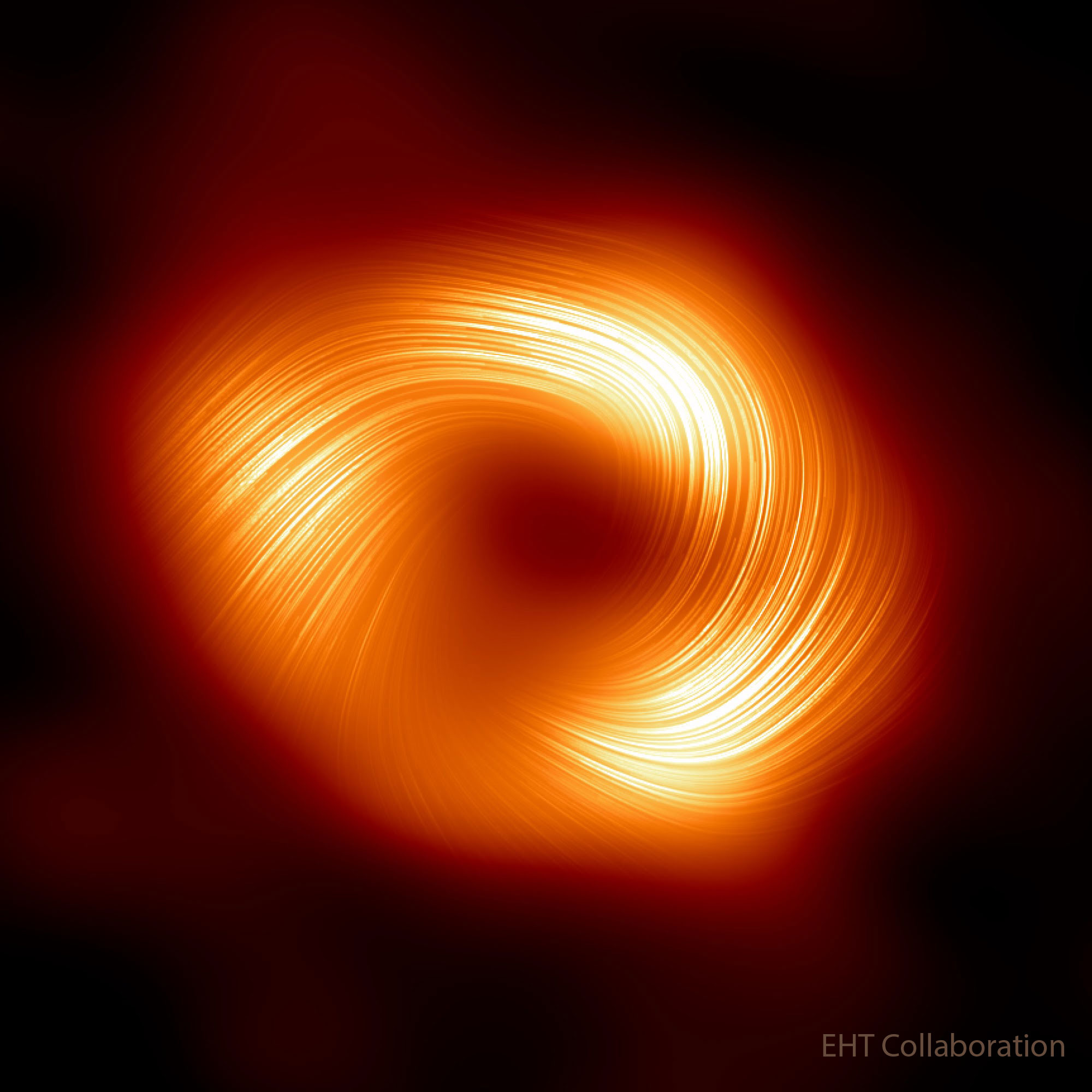
Figure 4: Reconstruction of the magnetic field lines of the supermassive black hole Sgr A$^{*}$. From the EHT collaboration.
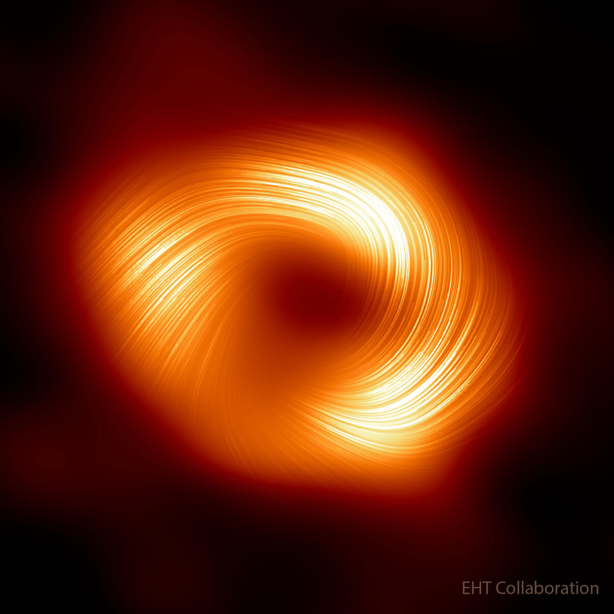
In GR, the uniqueness theorems state that any stationary black hole is described by the Kerr metric, characterized by its mass and spin alone (“black holes have no hair”). Alternative theories can predict hairy black holes or different near-horizon geometries, making black-hole observations a null test of the Kerr hypothesis.
The Event Horizon Telescope (EHT), a global millimetre-VLBI network, imaged the black-hole “shadow” of M87$*$ (2019) and Sgr A$*$ (2022). Photons passing within the critical impact parameter $b_c = \sqrt{27}\,GM/c^2$ (for Schwarzschild) are captured, leaving a dark region of angular diameter $\simeq 10.4\,GM/(c^2D)$ surrounded by a bright ring. For Sgr A, the mass-to-distance ratio is known independently from stellar orbits, making the comparison a genuine test: the measured ring agrees with the Kerr prediction at the $\sim 10\%$ level. Complementary strong-field probes of the same object come from the GRAVITY interferometer, which measured the gravitational redshift and the Schwarzschild precession of the star S2 around Sgr A.
Further reading an watching
- T. Baker - Tests of gravity - Michigan Cosmology Summer School 2025 lectures
- C.M. Will -The Confrontation between General Relativity and Experiment - 2014 - Living reviews in relativity .
- C. M. Will - theory and experiment in gravitational physics - second edition 2018 - Cambridge University Press.
- N. Yunes et al - Gravitational-Wave Tests of General Relativity with Ground-Based Detectors and Pulsar-Timing Arrays - 2024.
- Berti et al - 2015 - Testing General Relativity with Present and Future Astrophysical Observations.
- Barack et al - 2019 - Black holes, gravitational waves and fundamental physics: a roadmap.