Empirical validation of general relativity III: Gravity and cosmology
At least three reasons make cosmology a unique laboratory for gravitation:
- First, cosmology probes gravity in a regime inaccessible to all the tests seen so far: the lowest curvature regime, a completely different corner of parameter space than the Solar System or binary pulsars (see again Figure 1 of our lecture on local and astrophysical constraints; cosmological tests sit in the lower part of both panels). Furthermore, cosmology probes gravity on the largest possible scales ($\sim$ Gpc) and during the earliest phases of our Universe, hence providing the largest possible lever arms on the universality of physical laws and on principles such as the LPI.
- Second, low-density cosmological environments are precisely where screening mechanisms (chameleon, Vainshtein), which we will discuss later, are inefficient. Screening mechanisms are modifications of gravity that manifest themselves only in low-density environments, and not in high-density ones such as the Solar System. Hence, theories carefully tuned to modify GR while surviving the sharp local tests can still be caught in cosmology.
- Third, in order to account for its observables, cosmology needs the dark sector: dark matter and dark energy. These components are detected only through their gravitational effects, using GR as the translating dictionary. This is particularly exciting, as these two components are clearly the most mysterious and the least well understood parts of contemporary fundamental physics. They provide connections between particle physics and gravity, and it is yet unclear how such components may fit into this framework (new particles/fields, modifications of gravity, …).
What can be probed by cosmology?
Background cosmology
Friedmann equations
Cosmology rests on the cosmological principle: on large scales the Universe is homogeneous (invariant under spatial translations) and isotropic (invariant under spatial rotations) with respect to a specific frame known as the comoving frame. We consider a spherical coordinate chart $(t,r,\theta,\varphi)$ associated to this frame and centered (arbitrarily) on our Galaxy. The coordinates are chosen to be comoving: galaxies at rest with respect to the cosmic fluid keep the same values of their coordinates forever. Their physical separations nevertheless evolve, through the so-called scale factor $a(t)$, such that the physical distance $d$ of an object is recovered as $d=a(t)r$ (for a flat Universe; for curved spatial sections $r$ is replaced by the proper radial coordinate $\chi = \int_0^r \text{d}r’/\sqrt{1-K r’^2}$). We choose that, today at $t=t_0$, $a(t_0)=1$.
The most general metric compatible with these symmetries is the so-called Friedmann–Lemaître–Robertson–Walker (FLRW) metric, expressed in our comoving coordinate chart as:
\[\boxed{g = -c^2\,\text{d}t\otimes \text{d}t + a^2(t)\left[\frac{\text{d}r\otimes\text{d}r}{1- K r^2} + r^2\,\left(\text{d}\theta\otimes\text{d}\theta + \sin^2\theta\, \text{d}\varphi\otimes\text{d}\varphi\right)\right]}\]Let us stress that this form follows from the symmetries alone: no field equation has been used yet. The constant $K$, of dimension (length)$^{-2}$, measures the spatial curvature of the Universe as a whole, its sign selecting the geometry of the spatial sections: hyperbolic ($K<0$), Euclidean ($K=0$) or spherical ($K>0$). (The common normalization $K\in{-1,0,+1}$ is possible only at the price of releasing our convention $a(t_0)=1$.) For a flat Universe, $K=0$, the metric reduces, in a Cartesian comoving chart $(t,x,y,z)$, to:
\[\boxed{g = -c^2\,\text{d}t\otimes \text{d}t + \sum_i a^2(t)\, \text{d}x^i\otimes\text{d}x^i}\]That is, a Minkowski metric whose spatial sections are stretched by the scale factor $a(t)$. In terms of the conformal time $\text{d}\tilde{\eta} = \text{d}t/a$, it even becomes $g = a^2(\tilde{\eta})\,g_{\text{Mink}}$: the flat FLRW metric is conformally Minkowskian — a fact we will use again, since physics that is conformally invariant (such as the propagation of light) is blind to the expansion. Today, measurements constrain the Universe to be flat to a few per mille, \(\Omega_K \equiv -\frac{K c^2}{H_0^2} = 0.0007 \pm 0.0019\) where \(H_0 \equiv \dot{a}(t_0)\), from Planck 2018 VI, and we will very often set $K=0$, as it drastically simplifies the calculations.
The symmetries also force the matter content to take the perfect-fluid form, with energy density $\rho c^2$ and pressure $p$ functions of $t$ only. As we saw in our first lecture, this means:
\[T_{\mu\nu} = \left(\rho + \frac{p}{c^2}\right)u_\mu u_\nu + p\, g_{\mu\nu},\]with $u^\mu$ the four-velocity of comoving observers. It is only now that we invoke a theory of gravity: plugging these into the Einstein equation (D1), one obtains the two Friedmann equations:
\[\boxed{\left(\frac{\dot a}{a}\right)^2 = \frac{8\pi G}{3}\rho - \frac{K c^2}{a^2}}\] \[\boxed{\frac{\ddot{a}}{a}= -\frac{4\pi G}{3}\left(\rho + \frac{3p}{c^2}\right)}\]These two equations describe the large-scale evolution of the Universe, which is called the background cosmology. Note the division of labour: symmetry fixed the form of $g$ and $T_{\mu\nu}$; the theory of gravity only determines the dynamics of $a(t)$. This is why the FLRW form survives in modified theories of gravity — as long as the cosmological principle remains satisfied — with only the Friedmann equations being deformed.
Derivation from the Einstein equations
We derive the $K=0$ case explicitly and quote the curved generalization at the end. Coordinates are $(t,x^i)$, so $g_{00} = -c^2$, $g_{ij} = a^2(t)\,\delta_{ij}$, and $g^{00} = -1/c^2$, $g^{ij} = a^{-2}\delta^{ij}$.
From \(\Gamma^{\rho}_{\mu\nu} = \tfrac12 g^{\rho\sigma}(\partial_\mu g_{\sigma\nu} + \partial_\nu g_{\sigma\mu} - \partial_\sigma g_{\mu\nu})\), the only non-vanishing derivatives are \(\partial_t g_{ij} = 2a\dot a\,\delta_{ij}\), so the only non-zero symbols are:
\[\Gamma^{t}_{ij} = -\tfrac12 g^{00}\,\partial_t g_{ij} = \frac{a\dot a}{c^2}\,\delta_{ij}, \qquad \Gamma^{i}_{tj} = \tfrac12 g^{ik}\,\partial_t g_{kj} = \frac{\dot a}{a}\,\delta^{i}_{j}.\]We also compute the useful trace \(\Gamma^{\mu}_{\mu t} = \Gamma^i_{it} = 3\dot a/a\).
Now, the Ricci tensor. With \(R_{\mu\nu} = \partial_\rho\Gamma^{\rho}_{\mu\nu} - \partial_\nu\Gamma^{\rho}_{\rho\mu} + \Gamma^{\rho}_{\rho\lambda}\Gamma^{\lambda}_{\mu\nu} - \Gamma^{\rho}_{\nu\lambda}\Gamma^{\lambda}_{\rho\mu}\), and using \(\Gamma^{\rho}_{00}=0\), we get:
\[R_{00} = -\partial_t \Gamma^{i}_{it} - \Gamma^{i}_{tj}\Gamma^{j}_{it} = -\partial_t\!\left(3\frac{\dot a}{a}\right) - 3\left(\frac{\dot a}{a}\right)^2 = -3\left(\frac{\ddot a}{a} - \frac{\dot a^2}{a^2}\right) - 3\frac{\dot a^2}{a^2} = -3\,\frac{\ddot a}{a}.\]And, using the homogeneity hypothesis to kill all spatial derivatives:
\[R_{ij} = \partial_t\Gamma^{t}_{ij} + \Gamma^{\mu}_{\mu t}\Gamma^{t}_{ij} - \Gamma^{k}_{it}\Gamma^{t}_{jk} - \Gamma^{t}_{ik}\Gamma^{k}_{jt} = \left[\frac{\dot a^2 + a\ddot a}{c^2} + \frac{3\dot a^2}{c^2} - \frac{2\dot a^2}{c^2}\right]\delta_{ij} = \frac{a\ddot a + 2\dot a^2}{c^2}\,\delta_{ij}.\]We now compute the Ricci scalar and the Einstein tensor:
\[R = g^{00}R_{00} + g^{ij}R_{ij} = \frac{3\ddot a}{c^2 a} + \frac{3(a\ddot a + 2\dot a^2)}{c^2a^2} = \frac{6}{c^2}\left(\frac{\ddot a}{a} + \frac{\dot a^2}{a^2}\right).\] \[G_{00} = R_{00} - \tfrac12 R\,g_{00} = -3\frac{\ddot a}{a} + 3\left(\frac{\ddot a}{a}+\frac{\dot a^2}{a^2}\right) = 3\left(\frac{\dot a}{a}\right)^2,\] \[G_{ij} = R_{ij} - \tfrac12 R\,g_{ij} = \frac{a\ddot a + 2\dot a^2 - 3a\ddot a - 3\dot a^2}{c^2}\,\delta_{ij} = -\frac{a^2}{c^2}\left(2\frac{\ddot a}{a} + \frac{\dot a^2}{a^2}\right)\delta_{ij}.\]Comoving observers have $u^\mu = (1,0,0,0)$ (normalized: $g_{\mu\nu}u^\mu u^\nu = -c^2$), so $u_t = -c^2$ and
\[T_{00} = \left(\rho+\frac{p}{c^2}\right)c^4 + p\,(-c^2) = \rho c^4, \qquad T_{ij} = p\,g_{ij} = p\,a^2\delta_{ij}.\]We finally reach the two Friedmann equations. The Einstein equation $G_{\mu\nu} = \frac{8\pi G}{c^4}T_{\mu\nu}$ gives:
$00$-component:
\[3\left(\frac{\dot a}{a}\right)^2 = \frac{8\pi G}{c^4}\,\rho c^4 \quad\Longrightarrow\quad \left(\frac{\dot a}{a}\right)^2 = \frac{8\pi G}{3}\rho.\]$ij$-component:
\[-\frac{a^2}{c^2}\left(2\frac{\ddot a}{a} + \frac{\dot a^2}{a^2}\right) = \frac{8\pi G}{c^4}\,p\,a^2 \quad\Longrightarrow\quad 2\frac{\ddot a}{a} + \left(\frac{\dot a}{a}\right)^2 = -\frac{8\pi G}{c^2}\,p.\]Substituting the first into the second:
\[\frac{\ddot a}{a} = -\frac{4\pi G}{3}\left(\rho + \frac{3p}{c^2}\right).\]Note where the pressure enters: through the trace part of the Einstein equation (the $ij$-sector), which has no Newtonian counterpart — this is the “pressure gravitates” term discussed in the main text.
For $K\neq 0$ the spatial slices are curved, contributing the spatial curvature scalar $R^{(3)} = 6K/a^2$; the computation (heavier, because the spatial Christoffels no longer vanish) modifies only $G_{00} \to 3(\dot a^2 + K c^2)/a^2$ and correspondingly the $ij$-sector, yielding the $-K c^2/a^2$ term in the first Friedmann equation and leaving the second unchanged. Including $\Lambda$ in (D1) adds $+\Lambda c^2/3$ to the first equation and $+\Lambda c^2/3$ to the second (equivalently: treat it as a fluid with $\rho_\Lambda = \Lambda c^2/8\pi G$, $p_\Lambda = -\rho_\Lambda c^2$).
The Bianchi identity $\nabla_\mu G^{\mu\nu} = 0$ enforces $\nabla_\mu T^{\mu\nu} = 0$, whose $t$-component is the continuity equation
\[\dot\rho = -3\frac{\dot a}{a}\left(\rho + \frac{p}{c^2}\right).\]Any two of {Friedmann I, Friedmann II, continuity} imply the third — which is why deriving Friedmann II by differentiating Friedmann I (as in the Newtonian discussion below) is legitimate once the relativistic continuity equation is granted.
Densities
As commonly done in cosmology, we introduce the Hubble parameter $H \equiv \dot{a}/a$, the critical density today $\rho_c \equiv 3H_0^2/(8\pi G)$, and the density parameter of each component,
\[\Omega_i \equiv \frac{\rho_{i,0}}{\rho_c},\]where $\rho_{i,0}$ is its present-day density. Curvature and the cosmological constant are included in this sum by treating them as effective fluids. Furthermore, one generally assumes that every component is described by a simple barotropic equation of state with constant parameter $w_i$, relating pressure to energy density as $P_i = w_i \rho_i$ (we now set $c=1$; see the units box above). For baryonic and cold dark matter $w_i \simeq 0$, for radiation and relativistic species $w_i = 1/3$, for a cosmological constant $w_i = -1$, and for curvature $w_i = -1/3$. All these choices are justified in the supplement below.
The continuity equation, which follows from the conservation of the stress-energy tensor \(\nabla_\mu T^{\mu\nu} = 0\), gives in a FLRW background (proof below):
\[\boxed{\dot{\rho} + 3H(\rho + P) = 0,}\]translating the local conservation of the total energy density ($\rho = \sum_i \rho_i$). It can then be integrated, for constant $w_i$ and non-interacting fluids, to give the scaling of each density with the scale factor:
\[\rho_i(a) = \rho_{i,0}\, a^{-3(1+w_i)}, \qquad \text{i.e.} \qquad \frac{\rho_i(a)}{\rho_c} = \Omega_i\, a^{-3(1+w_i)},\]where we used $a(t_0) = 1$. With these notations, the two Friedmann equations become:
\[\boxed{\;\frac{H^2}{H_0^2} = \sum_i \Omega_i\, a^{-3(1+w_i)}\;}\] \[\boxed{\;\frac{\dot{H}}{H_0^2} + \frac{H^2}{H_0^2} = -\frac{1}{2}\sum_i \Omega_i\,(1+3w_i)\,a^{-3(1+w_i)}\;}\]The second equation is the acceleration equation, obtained from $\ddot{a}/a = \dot{H} + H^2$. Note that curvature drops out of it automatically from the second equation, since $1+3w_K = 0$. The first Friedmann equation evaluated today, at $t = t_0$ and $a = 1$, gives the closure equation
\[\sum_i \Omega_i = 1, \qquad \text{with} \qquad \Omega_K \equiv -\frac{K}{H_0^2 a_0^2} = 1 - \sum_{i \neq K}\Omega_i ,\]allowing us to interpret the $\Omega_i$ as the fractions of energy carried by each component today.
Everywhere above, the $\Omega_i$ are constant parameters, quantifying the energy density contribution of a component at $t=t_0$. In this lecture we will also use the common shorthand
\[\Omega_i(a) \;\equiv\; \frac{\rho_i(a)}{\rho_c(a)}, \qquad\text{with}\qquad \rho_c(a) \equiv \frac{3H^2(a)}{8\pi G}\]for the instantaneous fraction of the energy budget carried by component $i$.
Expression for the densities
Consider the $\nu = 0$ component of the conservation equation $\nabla_\mu T^{\mu\nu} = 0$ for a perfect fluid $T^{\mu\nu} = (\rho + P)u^\mu u^\nu + P g^{\mu\nu}$. The covariant divergence of a rank-2 contravariant tensor carries one Christoffel term per upper index:
\[\nabla_\mu T^{\mu 0} = \partial_\mu T^{\mu 0} + \Gamma^{\mu}_{\mu\lambda}T^{\lambda 0} + \Gamma^{0}_{\mu\lambda}T^{\mu\lambda}.\]The only non-vanishing Christoffel symbols in a flat FLRW metric (cosmic time, $c=1$) are:
\[\Gamma^{0}_{ij} = a\dot{a}\,\delta_{ij}, \qquad \Gamma^{i}_{0j} = \Gamma^{i}_{j0} = H\,\delta^{i}_{\ j},\]with $H = \dot{a}/a$. For a perfect fluid at rest in the comoving frame, $u^\mu = (1,0,0,0)$, the non-zero components of the stress-energy tensor are
\[T^{00} = \rho, \qquad T^{ij} = P\,g^{ij} = \frac{P}{a^2}\,\delta^{ij}, \qquad T^{0i} = 0.\]Evaluating the three terms separately, and using \(\Gamma^{\mu}_{\mu\lambda} = \partial_\lambda \ln\sqrt{-\vert g\vert}\) (prooved in the first lecture) with $\sqrt{-\vert g\vert} = a^3$, so that $\Gamma^\mu_{\mu 0} = 3H$:
\[\partial_\mu T^{\mu 0} = \dot\rho, \qquad \Gamma^{\mu}_{\mu\lambda}T^{\lambda 0} = 3H\rho, \qquad \Gamma^{0}_{\mu\lambda}T^{\mu\lambda} = \Gamma^0_{ij}T^{ij} = a\dot a\,\delta_{ij}\frac{P}{a^2}\delta^{ij} = 3HP,\]from which we obtain:
\[\boxed{\dot{\rho} + 3H(\rho + P) = 0.}\]The two contributions have a transparent reading: $3H\rho$ is pure volume dilution, and $3HP$ is the work done by the fluid against the expansion. Equivalently, this is the first law of thermodynamics for adiabatic expansion, $\text{d}(\rho a^3) = -P\,\text{d}(a^3)$. Inserting $P = w\rho$ with $w$ constant yields
\[\text{d}\ln\rho = -3(1+w)\,\text{d}\ln a,\]which can be integrated to obtain (using $a(t_0)=1$):
\[\rho = \rho_0\, a^{-3(1+w)}.\]Each component of the Universe evolves this way, in the limit where the fluids do not interact with one another:
-
Radiation, $w = 1/3$. The electromagnetic stress-energy tensor, which can be computed from the electromagnetic Lagrangian, is traceless, $T^\mu{}_{\mu} = -\rho + 3P = 0$, giving $P = \rho/3$. The kinetic theory of gases gives the same result for any ultra-relativistic gas with $v \to c$ and $E = pc$, and so does statistical physics applied to blackbody radiation. Hence $\rho_r \propto a^{-4}$ — three powers from volume dilution, one from the redshifting of each photon’s energy.
-
Non-relativistic matter, $w \simeq 0$. For a gas of particles with $v \ll c$, the pressure $P \sim \tfrac{1}{3}\rho\langle v^2\rangle/c^2$ is suppressed relative to the rest-mass energy density by $\langle v^2\rangle/c^2$. For cold dark matter this is utterly negligible ($w \lesssim 10^{-10}$), so $w = 0$ and \(\rho_m \propto a^{-3}\): pure volume dilution. Here and throughout, \(\rho_m\) denotes the total non-relativistic matter, cold dark matter and baryons, since after decoupling the two fall into the same potential wells and are indistinguishable gravitationally.
-
Cosmological constant, $w = -1$. A $\Lambda$ term in the Einstein equation contributes $T_{\mu\nu}^{(\Lambda)} = -\frac{\Lambda}{8\pi G}g_{\mu\nu}$. Matching to the perfect-fluid form requires $\rho_\Lambda = -P_\Lambda = \Lambda/(8\pi G)$, i.e. $w = -1$. More generally, any Lorentz-invariant vacuum must have $T_{\mu\nu} \propto g_{\mu\nu}$, since $g_{\mu\nu}$ is the only available invariant tensor. Then $\rho_\Lambda \propto a^0$: constant, as required.
-
Curvature, $w = -1/3$. Curvature is not a fluid; this is a formal bookkeeping device. Moving the $-K/a^2$ term of the Friedmann equation to the right-hand side defines $\rho_K \equiv -\frac{3K}{8\pi G a^2} \propto a^{-2}$, and matching $a^{-3(1+w)} = a^{-2}$ gives $w = -1/3$. Consistently, $1 + 3w_K = 0$, so curvature neither accelerates nor decelerates the expansion.
Newtonian vs GR cosmology
One might naively think that GR is absolutely required in order to build a coherent cosmological model accounting for the expansion of the Universe. It is not: at the background level, Newtonian and GR cosmology are indistinguishable. Indeed, applying Newton’s laws to a homogeneous expanding ball of dust reproduces exactly the Friedmann equations.
Consider a homogeneous ball of density $\rho(t)$ and a test shell of radius $r(t) = a(t)\,x$, with $x$ a fixed (comoving) label. By Gauss’s theorem, only the interior mass $M = \frac{4}{3}\pi r^3 \rho$ acts on the shell:
\[\ddot r = -\frac{GM}{r^2} = -\frac{4\pi G}{3}\rho\, r.\]In terms of $a$, this equation is
\[\boxed{\frac{\ddot{a}}{a}= -\frac{4\pi G}{3}\rho} \qquad \text{(dust only)}\]in which one recognizes the second Friedmann equation — for pressureless matter. Multiplying by $\dot r$ and integrating once (legitimate because $M$ is conserved for dust), with the integration constant written as $-\frac{1}{2}K c^2 x^2$:
\[\frac{1}{2}\dot r^2 - \frac{GM}{r} = -\frac{1}{2}K c^2x^2 \quad\Longrightarrow\quad \boxed{\left(\frac{\dot a}{a}\right)^2 = \frac{8\pi G}{3}\rho - \frac{K c^2}{a^2}}\]which is the first Friedmann equation, with the spatial curvature emerging as a mere integration constant (the shell’s total energy). Measurements of $H(z)$ alone — supernovae, BAO — therefore test the content of the Friedmann equation, not the theory of gravity behind it.
You may however have noticed that the Newtonian second Friedmann equation is incomplete: the $3p/c^2$ term is missing. It is entirely negligible for matter, but not for relativistic species. Hence there is one crucial thing that cannot be reproduced in Newtonian gravity: the gravitational effect of light. The early phase of radiation domination, for instance, has no Newtonian explanation. To properly test the nature of gravity itself, we must go beyond the background: to perturbations, and above all to light.
Let’s finally talk about $\Lambda$
So far we have barely discussed the cosmological constant $\Lambda$, which appears in the Einstein equations and the Einstein–Hilbert action (D1). As its name indicates, a lecture on cosmology is the right place to discuss it.
Observations of type Ia supernovae revealed that the expansion of the Universe is accelerating today (Riess et al. 1998; Perlmutter et al. 1999). Within GR, acceleration requires a component with sufficiently negative pressure: from the second Friedmann equation, $\ddot a > 0$ demands $\rho + 3p/c^2 < 0$, i.e. an equation of state $w \equiv p/(\rho c^2) < -1/3$. Whatever plays this role is called dark energy.
The most economical candidate is a non-zero cosmological constant $\Lambda$, which behaves as a perfect fluid with $w = -1$ exactly. And $\Lambda$ is not an arbitrary addition to GR: $\Lambda g_{\mu\nu}$ is the only term besides the Einstein tensor that can appear in second-order, divergence-free field equations in 4D — if anything, setting it to zero is what would require justification. Historically, Einstein introduced it in 1917 for the opposite purpose, to allow a static universe; after Hubble’s discovery of the expansion he reportedly called it his “biggest blunder” (a quote transmitted by Gamow, and possibly apocryphal).
The observed acceleration requires
\[\Lambda \simeq 1.1\times 10^{-52}\ m^{-2}, \qquad \text{i.e.}\qquad \rho_\Lambda c^2 = \frac{\Lambda c^4}{8\pi G} \simeq 5\times 10^{-10}\ \text{J.m}^{-3} \simeq (2.3\ \text{meV})^4.\]On the other hand, in quantum field theory the vacuum carries an energy density, and Lorentz invariance forces it to gravitate exactly like a cosmological constant, $T_{\mu\nu}^{\text{vac}} = -\rho_{\text{vac}}c^2\, g_{\mu\nu}$. A naive estimate with a Planck-scale cutoff gives $\rho_{\text{vac}} \sim m_{\text{Pl}}^4$, some $10^{120}$ times too large (still $\sim 10^{58}$ times too large with a conservative TeV cutoff — the problem does not hinge on trusting quantum gravity). This is the cosmological constant problem, arguably the worst fine-tuning in physics (Weinberg 1989; pedagogical reviews: Martin 2012, Padilla 2015). It comes in two layers: the old problem (why doesn’t the vacuum gravitate at its QFT value?) and the coincidence problem (why is $\rho_\Lambda$ comparable to \(\rho_m\) precisely today?).
One might object that this is a problem of quantum field theory rather than of our theory of gravity. But the problem lives exactly at their interface: gravity is the only interaction that responds to the absolute zero-point of energy — everywhere else in physics, only energy differences are observable and the vacuum can be renormalized away. This is why modifying the gravity side is a legitimate strategy, and several of the theories we will meet later are designed to do so. However, there is a famous obstruction to this approach: a no-go theorem by Weinberg shows that this is not easy, as no dynamical adjustment mechanism based on standard assumptions can relax $\Lambda$ to zero without fine-tuning — every proposal must break one of its hypotheses. For more, see e.g. Brax (2018).
We note that the question “is dark energy exactly $\Lambda$?” is being tested by measuring $w(z)$: intriguingly, recent DESI BAO measurements combined with CMB and supernovae show a $\sim 3$–$4\sigma$ preference for an evolving equation of state (DESI DR2, 2025), though the robustness of this hint is actively debated (e.g. Wang & Mota (2025)). If confirmed, $\Lambda$ alone would be excluded — and the gravity-versus-dark-energy question of this lecture would become the central problem of cosmology.
And how about dark matter?
Understanding the nature of dark matter is perhaps the most exciting question of all: contrary to dark energy, dark matter has no simple candidate on either side of our canonical theories — the standard model of particle physics contains no viable particle for it (standard model neutrinos are too light and too fast), and, as we will see, no simple modification of gravity accounts for all the evidence either. And the evidence is overwhelming, spanning every scale and epoch: galaxy rotation curves stay flat where Newtonian gravity sourced by visible matter predicts a Keplerian decline (Rubin & Ford 1970), cluster velocity dispersions are far too large for the visible mass (Zwicky’s original 1933 observation, which coined dunkle Materie), weak lensing maps require deeper potentials than baryons provide, the relative heights of the CMB acoustic peaks demand a non-baryonic pressureless component with $\Omega_c h^2 \simeq 0.120$, and structure formation needs it: baryonic perturbations, frozen at $\sim 10^{-5}$ until recombination, could not have grown into galaxies by today without pre-existing potential wells dug by a component that decoupled from the photons much earlier. Note again that every single one of these detections is gravitational. Either a new matter component exists, or the gravitational theory has to be revised.
Some proposed modifications of gravity, such as that of Milgrom (1983), invoke a modification of the law of gravity below a universal acceleration scale $a_0 \simeq 1.2\times 10^{-10}$ m s$^{-2}$ — MOdified Newtonian Dynamics (MOND): for $a \ll a_0$, the true acceleration satisfies $a \simeq \sqrt{a_N\, a_0}$, with $a_N$ the Newtonian prediction. Two striking successes follow. First, flat rotation curves are automatic: $v^4 = GM_b\,a_0$. Second — and this was a genuine prediction, later confirmed with remarkably small scatter — the baryonic Tully–Fisher relation $v^4 \propto M_b$, and more generally a tight universal relation between the observed acceleration and the one sourced by baryons alone (McGaugh et al. 2016). Whatever dark matter is, it must explain why one can predict a galaxy’s dynamics from its baryons alone with essentially no scatter. Intriguingly, $a_0 \sim cH_0/6$: nobody knows whether this is a deep clue or numerology. To be confronted with relativistic tests, however, MOND must be embedded in a relativistic theory — Bekenstein’s TeVeS (2004) being the classic attempt, built precisely from the two-metric and disformal structure (light must bend more than the baryons allow, so the matter metric must differ from the gravitational one). We will return to this in later lectures.
Such theories face severe challenges. The merging cluster 1E 0657−56, known as the Bullet Cluster, is the emblematic one: the collision has separated the components. The hot X-ray gas — which contains most of the baryonic mass — was slowed by ram pressure and sits in the middle, while the weak-lensing mass reconstruction shows that the potential wells coincide instead with the two galaxy concentrations that flew through (Clowe et al. 2006). This is devastating for theories in which gravity is sourced by baryons alone, however modified: the mass is simply not where the baryons are. It is, on the other hand, exactly what a collisionless matter component predicts. Furthermore, explaining the acoustic peaks of the CMB, or the BAO scale with baryons only is a major challenge for MOND like theories as it requires a fluid of coupled baryons and photons oscillating in deeper dark matter wells.
MOND-like phenomenology thus works remarkably well at galaxy scales and poorly beyond: clusters still require missing mass even within MOND, and the CMB is its hardest test — for two decades no MOND-like theory could produce the observed acoustic peaks without dark matter. It is a measure of how sharp this test is that constructing a counter-example took until Skordis & Złośnik (2021), whose relativistic MOND fits the CMB and matter spectra — at the price of a carefully engineered additional field content (and having survived the $c_{\text{gw}}$ test of GW170817 by construction). The current balance of evidence thus favours a particle: a single collisionless component simultaneously explains galaxies (imperfectly — the tight baryon–dynamics relation remains a challenge), clusters, lensing, the CMB and structure formation. Note that this component need not be a fundamental particle (WIMP, axion, right-handed sterile neutrino, …): it could also consist of macroscopic objects such as primordial black holes. The viable candidates span some ninety orders of magnitude in mass — from fuzzy dark matter at $\sim 10^{-22}\ \text{eV}$ to black holes of tens of solar masses — a vivid reminder that gravity measures only the stress-energy content, not its identity. But no candidate has so far been detected non-gravitationally: particle candidates have evaded four decades of laboratory searches, while astronomical constraints (microlensing, gravitational-wave merger rates) now exclude primordial black holes as the dominant component over most of their mass range. Until such a detection occurs, the dark matter question remains, at bottom, a question about gravity: it is the assumption of GR that converts astronomical observations into the evidence for a new matter component.
Perturbations and growth in GR and beyond
Perturbation equations in General Relativity
We now turn to small perturbations around the flat FLRW background. This is where cosmology becomes a true laboratory for gravity: the background, as we saw, does not strongly select GR against an alternative such as Newtonian gravity, but the perturbations — how structures grow, and how light propagates through them — do. From here on we set $c=1$ in derivations, restoring it only in final boxed results.
The metric has 10 independent components; perturbing $g \to \bar g + \delta g$ introduces 10 functions. The symmetry of the background (in particular the symmetry of each spatial slice at fixed time) allows a powerful sorting: any $\delta g_{\mu\nu}$ decomposes into scalar (4 functions), vector (4) and tensor (2) pieces under spatial rotations (SO(3)), and — this is the decomposition theorem — at linear order the three sectors evolve independently. This is known as the SVT (scalar, vector, tensor) decomposition, and the objects are known as Bardeen scalars, vectors and tensors. Note that the Bardeen objects do not live in irreducible representations of the Lorentz group (as ordinary scalars, vectors and tensors in GR do), but in irreducible representations of the smaller group SO(3) of spatial rotations. Vectors are associated with vorticity and decay with the expansion, so we usually ignore them in cosmology; tensors are gravitational waves (they carry the $c_{\text{gw}}$ physics discussed previously); scalars are the ones sourced by density perturbations, and are of first importance in cosmology.
Not all 4 scalar functions are physical: perturbing the coordinates, $x^\mu \to x^\mu + \xi^\mu$, also shifts $\delta g$ (by the Lie derivative $-\mathcal{L}_\xi \bar g$) and can even generate fake perturbations. Example: slicing the perfectly homogeneous universe with a wiggly time coordinate $t \to t + T(t,\vec x)$ produces an apparent density perturbation $\delta\rho = -\dot{\bar\rho}\,T$ out of nothing. The scalar sector contains 2 gauge functions for 4 metric scalars: only 2 physical scalar potentials remain (the Bardeen potentials). One can either work with gauge-invariant combinations, or use the gauge freedom wisely. The Newtonian (longitudinal) gauge does the latter, bringing any perturbation to the form:
\[\boxed{g + \delta g \simeq -\left(1+\frac{2\Psi}{c^2}\right)c^2\,\text{d}t\otimes \text{d}t + a^2(t)\left[\left(1-\frac{2\Phi}{c^2}\right)\delta_{ij} + h_{ij}\right]\text{d}x^i \otimes \text{d}x^j}\]$\Psi$, the lapse function, is the analogue of the Newtonian potential: it drives the motion of non-relativistic matter and distorts the time geometry (recall from our previous lectures that in the Newtonian limit of GR, gravitation is entirely a geometry-of-time effect). $\Phi$ perturbs the spatial geometry and can be read as a local perturbation of the scale factor. In this gauge the two potentials coincide with the gauge-invariant Bardeen potentials, which is why it is the gauge of choice for physical interpretation. For a detailed construction, see chapters 5 and 6 of Baumann (2022). Note that many other gauges can be selected and may drastically simplify the equations depending on the problem. The Newtonian gauge is often preferred for pedagogy, as it is the one allowing an interpretation of the perturbations in Newtonian terms. Finally, $h_{ij}$ denotes the transverse–traceless tensor modes ($\partial^i h_{ij} = h^i{}_i = 0$), corresponding to the propagation of gravitational waves; we have dropped the vector perturbations because, as discussed above, they dilute away very rapidly in standard cosmology.
We can play the same game with the stress-energy tensor of cosmological fluids. Perturbing a fluid to first order (barred quantities are background values):
\[T^0{}_0 = -(\bar\rho + \delta\rho), \qquad T^0{}_i = (\bar\rho + \bar P)\,v_i, \qquad T^i{}_j = (\bar P + \delta P)\,\delta^i_j + \Pi^i{}_j,\]where $v^i$ is the peculiar (bulk) velocity of the fluid and $\Pi^i{}_j$ its traceless anisotropic stress. We define the density contrast $\delta \equiv \delta\rho/\bar\rho$, the equation of state $w = \bar P/\bar\rho$, and for each species the velocity divergence $\theta \equiv \partial_i v^i$. For a perfect fluid, $\Pi^i{}_j = 0$; in the real Universe the only notable anisotropic stress is that of free-streaming neutrinos and photons.
Let us now plug these perturbed objects into the Einstein equation and keep only the first-order terms. Linearizing $G_{\mu\nu} = 8\pi G\,T_{\mu\nu}$ around FLRW (full set in the box below) and combining its $00$ and $0i$ components, one obtains two remarkably simple statements, in Fourier space:
\[\boxed{\frac{k^2}{a^2}\,\Phi = -4\pi G\,\bar\rho\,\Delta}\] \[\boxed{\frac{k^2}{a^2}(\Phi - \Psi) = 12\pi G\,(\bar\rho+\bar P)\,\sigma \;\;\Longrightarrow\;\; \Phi = \Psi \;\;\text{if $\sigma=0$}}\]where $\sigma \propto \Pi$ is the scalar part of the anisotropic stress, $\bar\rho\Delta \equiv \sum_i \bar\rho_i\Delta_i$ runs over all species, and
\[\Delta \equiv \delta + 3\frac{aH}{k^2}(1+w)\,\theta\]is the comoving density contrast — the density contrast measured by observers comoving with the fluid. Three comments:
- The first equation generalizes the Newtonian Poisson equation — with a subtlety: written with $\Delta$ (not $\delta$), it is exact on all linear scales, not just sub-horizon. The velocity correction in $\Delta$ is negligible for $k \gg aH$ (sub-horizon), where $\Delta \simeq \delta$, and this is the regime where the naive Newtonian intuition applies.
- The second equation is the cosmological sibling of the PPN statement $\gamma = \beta = 1$: in GR, the two potentials differ only through anisotropic stress, which is negligible once neutrinos are subdominant. In modified gravity, $\Phi \neq \Psi$ generically even for perfect fluids: the gravitational slip $\eta \equiv \Phi/\Psi$ is thus a probe of modified gravity.
- The acceleration of non-relativistic particles responds to $\Psi$ only (their Euler equation is $\dot{\vec v} + H\vec v = -\vec\nabla\Psi/a$); photons respond to the sum $\Phi+\Psi$ (the Weyl potential, up to a factor 2). The whole strategy of cosmological tests of gravity is the large-scale version of the PPN investigation: measure the mass of structures once with matter (probing $\Psi$) and once with light (probing $\Phi+\Psi$), and check the two answers against each other.
Energy–momentum conservation $\nabla_\mu T^{\mu\nu} = 0$, linearized for cold matter, gives a continuity and an Euler equation (both derived in the box below). Both can be combined with the Poisson equation into the growth equation, which governs how structures assemble; because that equation and its solutions are the whole subject of the next section.
For the tensor perturbations, one obtains instead
\[\boxed{\ddot{h}_{ij} + 3H \dot{h}_{ij} + \frac{k^2}{a^2} h_{ij}=0}\]a wave equation for $h_{ij}$. This is the expanding space-time generalisation of the waves whose propagation velocity and possible damping (mass) are constrained by the previous discussion on gravitational wave experiments. In standard cosmology, scalar and tensor perturbations are decoupled at linear order: each propagates independently of the other. We will focus on scalar perturbations in this lecture and leave the tensor sector aside for now. We simply note that the study of a modified gravity model must be “holistic”: once you have selected your favorite model, you should compute the propagation of scalar perturbations and confront it with cosmological observables, but also consider the propagation of tensor perturbations and confront it with GW constraints. Furthermore, one should also look at the PPN parameters and at variations of constants and compare them with local and astrophysical data. Only such a complete analysis of a model can claim to be consistent. Constraining a modification of gravity is therefore hard work, and it is extremely difficult to find theories that are physically motivated, predict observationally interesting phenomena, and survive all the observational data.
More on perturbations and proof of the equations
We work in conformal time $\tilde{\eta}$ (${\text{d}}\tilde{\eta} = {\text{d}}t/a$), with $’ \equiv \partial_{\tilde{\eta}}$ and $\mathcal{H} \equiv a’/a = aH$, and in Fourier space ($\partial_i \to ik_i$); $c=1$. We discuss here only scalar perturbations.
Gauge transformations and the Newtonian gauge. The most general scalar perturbation of flat FLRW is
\[{\text{d}}s^2 = a^2(\tilde{\eta})\left\{-(1+2A)\,{\text{d}}\tilde{\eta}^2 + 2\,\partial_iB\;{\text{d}}\tilde{\eta}\,{\text{d}}x^i + \left[(1-2C)\delta_{ij} + 2\,\partial_i\partial_j E\right]{\text{d}}x^i{\text{d}}x^j\right\}.\]Under an infinitesimal coordinate change $\tilde{\eta} \to \tilde{\eta} + T$, $x^i \to x^i + \partial^i L$, the perturbations shift by $\delta g \to \delta g - \mathcal{L}_\xi \bar g$, which component by component reads:
\[A \to A - T' - \mathcal{H}T, \qquad B \to B + T - L', \qquad C \to C + \mathcal{H}T, \qquad E \to E - L,\]and for the matter, $\delta\rho \to \delta\rho - \bar\rho’\,T$ (the “fake density perturbation” of the main text). Choosing $L = E$ and $T = -B + E’$ sets $E = B = 0$: this defines the Newtonian gauge, with $\Psi \equiv A$, $\Phi \equiv C$, and the residual freedom is completely exhausted. The gauge-invariant Bardeen potentials,
\[\Psi_{\text{B}} \equiv A + \mathcal{H}(B-E') + (B-E')', \qquad \Phi_{\text{B}} \equiv C - \mathcal{H}(B-E'),\]reduce to $\Psi$ and $\Phi$ in this gauge: our potentials are physical, not coordinate artifacts.
The four scalar Einstein equations. We now linearize the Einstein tensor in this gauge. We simply give the final results, as this computation is straightforward but clearly tedious, and requires the perturbed Christoffels and Ricci tensor — see e.g. Ma & Bertschinger 1995, whose conventions we follow, or Baumann ch. 6. Equating to the perturbed $T_{\mu\nu}$ of the main text yields, in Fourier space:
\[\text{[00]}: \qquad k^2\Phi + 3\mathcal{H}\left(\Phi' + \mathcal{H}\Psi\right) = -4\pi G a^2\,\bar\rho\,\delta\] \[\text{[0i]}: \qquad k^2\left(\Phi' + \mathcal{H}\Psi\right) = 4\pi G a^2\,(\bar\rho + \bar P)\,\theta\] \[\text{[ij, trace]}: \qquad \Phi'' + \mathcal{H}(\Psi' + 2\Phi') + \left(2\mathcal{H}' + \mathcal{H}^2\right)\Psi + \frac{k^2}{3}(\Phi - \Psi) = 4\pi G a^2\,\delta P\] \[\text{[ij, traceless]}: \qquad k^2(\Phi - \Psi) = 12\pi G a^2 (\bar\rho + \bar P)\,\sigma\]where $(\bar\rho+\bar P)\sigma \equiv -(\hat k_i \hat k_j - \tfrac13\delta_{ij})\Pi^{ij}$. Only two of these are independent once the conservation equations below are imposed (Bianchi identity, as for the background).
Proof of the exact Poisson equation. Substitute [0i] into [00]:
\[k^2\Phi = -4\pi G a^2 \bar\rho\,\delta - 3\mathcal{H}\cdot\frac{4\pi Ga^2(\bar\rho+\bar P)\theta}{k^2} = -4\pi G a^2\,\bar\rho\left[\delta + 3\frac{\mathcal{H}}{k^2}(1+w)\,\theta\right] \equiv -4\pi Ga^2\bar\rho\,\Delta.\]No approximation was made: the combination $\Delta$ obeys the Poisson equation exactly. This is the reason $\Delta$ is introduced at all — it is precisely the combination that absorbs the $3\mathcal{H}(\Phi’+\mathcal{H}\Psi)$ term and restores the Newtonian form. Dividing by $a^2$ and restoring $\mathcal{H} = aH$ gives the boxed cosmic-time form of the main text. The [ij, traceless] equation is the boxed slip relation.
Conservation equations. The perturbation equations for a single fluid follow from the conservation of the perturbed stress-energy tensor, $\nabla_\mu T^\mu{}_\nu = 0$. In conformal time and in Newtonian gauge, its $\nu=0$ and $\nu=i$ components give respectively a continuity and an Euler equation:
\[\boxed{\;\delta' = -(1+w)\left(\theta - 3\Phi'\right) - 3\mathcal{H}\left(\frac{\delta P}{\bar\rho} - w\,\delta\right)\;}\] \[\boxed{\;\theta' = -\mathcal{H}\left(1-3w\right)\theta - \frac{w'}{1+w}\,\theta + \frac{k^2}{1+w}\,\frac{\delta P}{\bar\rho} + k^2\Psi - k^2\sigma\;}\]Two physical remarks. The $3\Phi’$ term is a volume effect: a local perturbation of the scale factor changes the volume in which particles are counted. So it is not quite true that matter “only feels $\Psi$” — its acceleration involves only $\Psi$, but its counted density also responds to $\Phi’$. Second, note the signs: for a growing overdensity ($\delta>0$, $\delta’>0$) the continuity equation gives $\theta<0$, i.e. converging infall, as it should. These two equations are the starting point of the growth equation derived in the next section.
Horizon bookkeeping. The ratio $\mathcal{H}/k$ organizes everything: super-horizon ($k \ll \mathcal{H}$), the potentials are constant for constant $w$ (and drop by a factor $9/10$ at the radiation–matter transition); sub-horizon ($k \gg \mathcal{H}$), $\Delta \to \delta$, the Poisson equation takes its Newtonian form, and the Newtonian intuition applies. All the “gravity is Newtonian inside the horizon” intuition of the previous sections is contained in these limits — while the observables of the next sections (lensing, RSD, ISW) are computed from the same two potentials without any such restriction.
A warning on conventions. Signs and factors in this subject vary between references: the sign of $\Phi$ in the metric, the sign of $\theta$, and cosmic vs. conformal time all differ between standard texts (Ma–Bertschinger, Dodelson, Baumann, Mukhanov). When comparing formulas across references — or coding them — always re-derive the Poisson sign convention first: here, an overdensity has $\Phi = \Psi < 0$ (a potential well), consistent with the weak-field limit $\Psi = \Phi = -GM/r$ of the Schwarzschild metric from the lecture on PPN parameters.
Cosmological deviation from GR: the $\mu,\Sigma,\eta$ parametrization
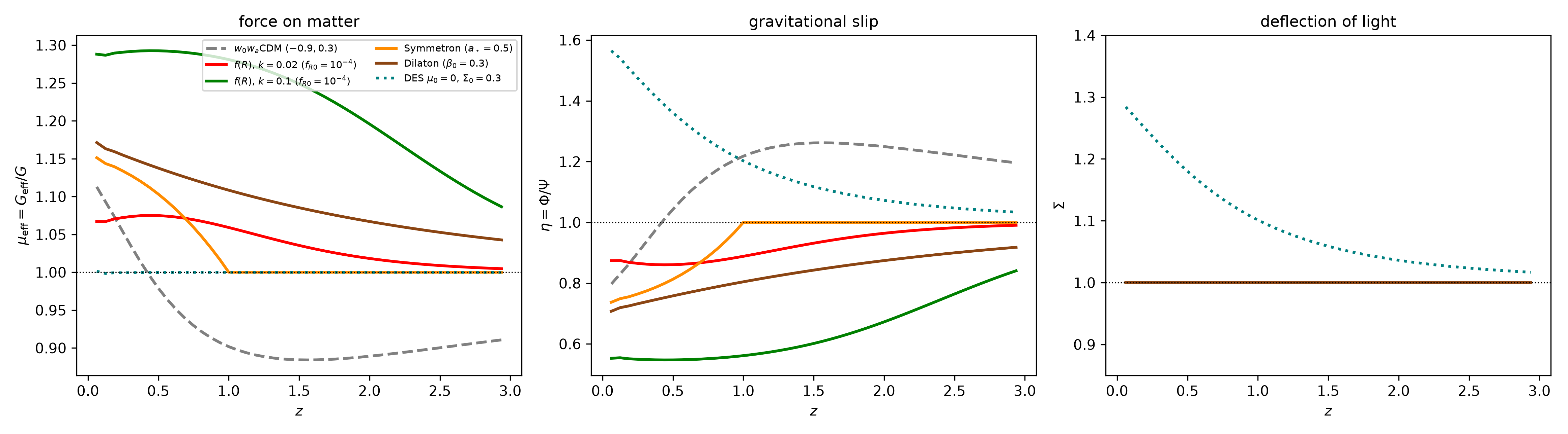
Figure 1: $\mu$, $\Sigma$ and $\eta$ for different modified gravity models implemented in MGCAMB. Derived in the associated notebook. No need to understand the details of the models yet. This figure will tell you how to interpret the different impact on cosmological observables of the various models.
In the same spirit as the PPN parameters, one can parametrize deviations from GR agnostically at the level of the perturbation equations:
\[\boxed{\frac{k^2}{a^2}\Psi = -4\pi G\,\mu(a,k)\,\bar\rho\Delta}, \qquad \boxed{\frac{k^2}{a^2}\left(\frac{\Phi+\Psi}{2}\right) = -4\pi G\,\Sigma(a,k)\,\bar\rho\Delta}, \qquad \boxed{\eta(a,k) \equiv \frac{\Phi}{\Psi}}\]$\mu$ modifies the force felt by matter (probed by redshift-space distortions, RSD, and by growth) and is exactly equivalent to a varying $G$ as discussed in the previous lecture; $\Sigma$ modifies the deflection of light (probed by lensing and ISW in the CMB); and $\eta$ is the gravitational slip. Only two of the three are independent, since dividing the first two boxed equations gives
\[\frac{\Sigma}{\mu} = \frac{(\Phi+\Psi)/2}{\Psi} = \frac{1+\eta}{2} \qquad\Longleftrightarrow\qquad \Sigma = \frac{\mu(1+\eta)}{2}.\]In GR, $\mu=\Sigma=\eta=1$. This is the cosmological analogue of the PPN pair $(\gamma,\beta)$: theory-agnostic knobs that any specific model maps onto. A useful complement, connecting to the previous lecture: standard sirens test the tensor sector on cosmological distances ($c_{\text{gw}}$, GW friction $d_L^{\text{gw}}/d_L^{\text{EM}}$), while $\mu,\Sigma,\eta$ test the scalar sector. Each theory of modified gravity has its own specific predictions for the triplet $(\mu, \Sigma, \eta)$, and computing them for a given model is a full piece of work in itself (which we will do in the next lectures) before one can confront them with experimental results.
In Figure 1, we display the $\mu$, $\Sigma$ and $\eta$ functions for different models implemented in MGCAMB (see associated notebook). Here and everywhere in this lecture, do not try to understand the meaning of the different models, this will be the topic of the following lectures. We will simply use them in everything that follows for illustration. We see that:
- All the MGCAMB models have $\mu \geq 1$, they thus introduce some kind of fifth force effect that increase the total strength of gravity. The $w_0-w_a$ model is not a modified gravity model but a dark energy parametrization plotted here for comparaison. We see that it is the only model which can produce $\mu \leq 1$, which is easy to understand, as dark energy acts as some kind of “anti-gravity” suppressing the growth of structure if its stronger than a cosmological constant (and the opposite otherwise).
- $\mu$, $\eta$ and $\Sigma$ can be different at different $k$. This is illustrated here only for the $f(R)$ model. Hence, based on $\mu$ we can say that $f(R)$ predicts a stronger fifth force for larger $k$ i.e. smaller scales.
- The orange curve, the “symmetron” model, activates itself at a critical redshift $z_\star$ and is otherwise invisible. This is some form of screening that will be discussed later.
- All the models implemented in MGCAMB do not interact with photons (they are said to be conformal, see this lecture). Hence, they introduce a change in the Newtonian potential $\Psi$ that is not there in the potential $\Phi$, such that $\Psi/\Phi$ is exactly the inverse of $\mu$. In all these models $\Sigma = 1$. We added a phenomenological model for which $\mu=0$ and $\Sigma\neq 0$ simply to illustrate the effect of a non zero $\Sigma$. Note that other non conformal modified gravity models, not implemented in MGCAMB (as some Horndeski models) can predict non-zero $\Sigma$ in a well motivated fashion, but they are severely constrained by data.
Growth of structure
We now cash in the first half of the strategy announced above: weighing structures with matter. The acceleration of non-relativistic tracers responds to $\Psi$ alone, so their growth history isolates $\mu$ — the lensing half, which isolates $\Sigma$, follows in the next section, and their ratio is the $E_G$ statistic.
Linear growth: general relativity
Combining the continuity and Euler equations obtained above with the Poisson equation, and specializing to non-relativistic matter, yields the linear growth equation. In cosmic time it reads
\[\boxed{\;\ddot{\Delta}_m + 2H\dot{\Delta}_m - 4\pi G\,\bar\rho_m\,\Delta_m = 0\;}\]where \(\Delta_m\) and \(\bar\rho_m\) refer to the total non-relativistic matter — cold dark matter and baryons, which after decoupling fall into the same potential wells and are gravitationally indistinguishable. Note the asymmetry that will recur throughout: the source term involves matter only, while the friction term involves the total expansion rate $H$, to which dark energy contributes.
Proof
We now look at the equations in the case where only matter and dark energy (\(\Lambda\)) contribute significantly to the evolution of the universe and all are decoupled. Dark energy disapear from most terms as \(\rho_\Lambda + p_\Lambda=0\) and $\Lambda$ being a constant it has no perturbations. Start from the conservation equations derived in the previous section, in conformal time. Now consider only pressureless matter ($w = w’ = \delta P = \sigma = 0$) leaves
\[\delta_m' = -\theta_m + 3\Phi' , \qquad \theta' = -\mathcal{H}\theta + k^2\Psi .\]Now, differentiate the comoving contrast $\Delta_m \equiv \delta_m + 3\mathcal{H}\theta/k^2$ directly and substitute both equations:
\[\Delta_{\rm m}' = -\theta + 3\left(\Phi' + \mathcal{H}\Psi\right) + \frac{3\left(\mathcal{H}'-\mathcal{H}^2\right)}{k^2}\,\theta .\]The $[0i]$ perturbed Einstein equation for matter only gives $3(\Phi’+\mathcal{H}\Psi) = 12\pi Ga^2\bar\rho_{\rm m}\theta/k^2$, while the background identities $\mathcal{H}’ = \mathcal{H}^2 + a^2\dot H$ and $\dot H = -4\pi G(\bar\rho + \bar P) = -4\pi G\bar\rho_{\rm m}$ give $3(\mathcal{H}’-\mathcal{H}^2)/k^2 = -12\pi Ga^2\bar\rho_{\rm m}/k^2$. The two cancel identically:
\[\boxed{\;\Delta_{\rm m}' = -\theta\;}\]The comoving contrast obeys the naive Newtonian continuity equation, with the volume term exactly absorbed — this is precisely what $\Delta$ was constructed to do. Differentiating once more, using the Euler equation, $\Psi = \Phi$, and the exact Poisson equation $k^2\Phi = -4\pi Ga^2\bar\rho_{\rm m}\Delta_{\rm m}$:
\[\Delta_{\rm m}'' + \mathcal{H}\,\Delta_{\rm m}' - 4\pi Ga^2\,\bar\rho_{\rm m}\,\Delta_{\rm m} = 0 ,\]For solving and interpreting this equation, the natural time variable is neither $t$ nor $\tilde{\eta}$ but the number of e-folds $N \equiv \ln a$. Writing $\partial_N \equiv \text{d}/\text{d}\ln a$ (not $’$, which remains reserved for conformal-time derivatives), it becomes
\[\boxed{\;\partial_N^2\Delta_m + \left(2 + \partial_N\ln H\right)\partial_N\Delta_m = \frac{3}{2}\,\Omega_m(a)\,\Delta_m\;}\]with \(\Omega_m(a) = \frac{\rho_m(a)}{\rho_c(a)}\) the instantaneous fraction of the total energy budget carried by matter, which falls from $1$ deep in matter domination to $\simeq 0.31$ today.
Three structural remarks before solving:
- The equation is the expanding-universe version of the Jeans instability: a damped oscillator in which the “restoring” term has the wrong sign, so perturbations grow rather than oscillate. The Hubble friction turns what would be exponential collapse into power-law growth.
- The friction coefficient $2 + \partial_N \ln H = \partial_N\left[\ln(a^2H)\right]$ is the Hubble drag: expansion fights collapse. Everything the background does to structure formation enters here, and only here.
- No $k$ appears anywhere. In GR, linear growth is scale-independent: every Fourier mode evolves with the same time dependence. Keep this in mind — it is exactly what modified gravity breaks, and the breaking is observable.
Since the equation contains no $k$, the solution factorizes into a scale-dependent amplitude times a universal function of time:
\[\Delta_m(a,\vec k) = D(a)\,\Delta_{m,0}(\vec k),\]which defines the growth factor $D$ (we keep only growing solutions doing so). We normalize $D(a{=}1)=1$, so that $\Delta_{m,0}$ is the present-day field. We also introduce the growth rate:
\[f=\frac{\text{d}\ln(D)}{\text{d}\ln(a)}\]Physically, $f$ measures how fast structure is currently assembling. The growth equation translates for the growth rate into the Riccati equation:
\[\boxed{\;\partial_N f + f^2 + \left(2 + \partial_N\ln H\right) f = \frac{3}{2}\,\Omega_{\rm m}(a)\;}\]Proof of the Riccati equation
Since $f \equiv \partial_N \ln D = 1/D \partial_N D$, we have immediately:
\[\partial_N D = f D, \qquad \partial_N^2 D = \left(\partial_N f + f^2\right)D .\]Substituting into the growth equation and dividing throughout by $D$ gives the Riccati equation for $f$:
\[\boxed{\;\partial_N f + f^2 + \left(2 + \partial_N\ln H\right) f = \frac{3}{2}\,\Omega_{\rm m}(a)\;}\]In standard $\Lambda$-CDM cosmology, the solution of this equation is very well approximated by a power-law \(f(a) \simeq \Omega_m(a)^{\gamma_g}\), with the growth index being \(\gamma_g = 6/11\) (for an analytical proof, see Wang & Steinhardt (1998)). Since $\gamma$ compresses the whole growth history into a single number, it is the most compact null test of GR available from structure growth. As the summary table at the end of this lecture records, current data give $\gamma_g = 0.633^{+0.025}_{-0.024}$, a $3.7\sigma$ preference for suppressed growth relative to the GR value $6/11$ (Nguyen, Huterer & Wen (2023)). Whether this survives scrutiny is one of the open questions this lecture is ultimately about.
Linear growth: modified gravity
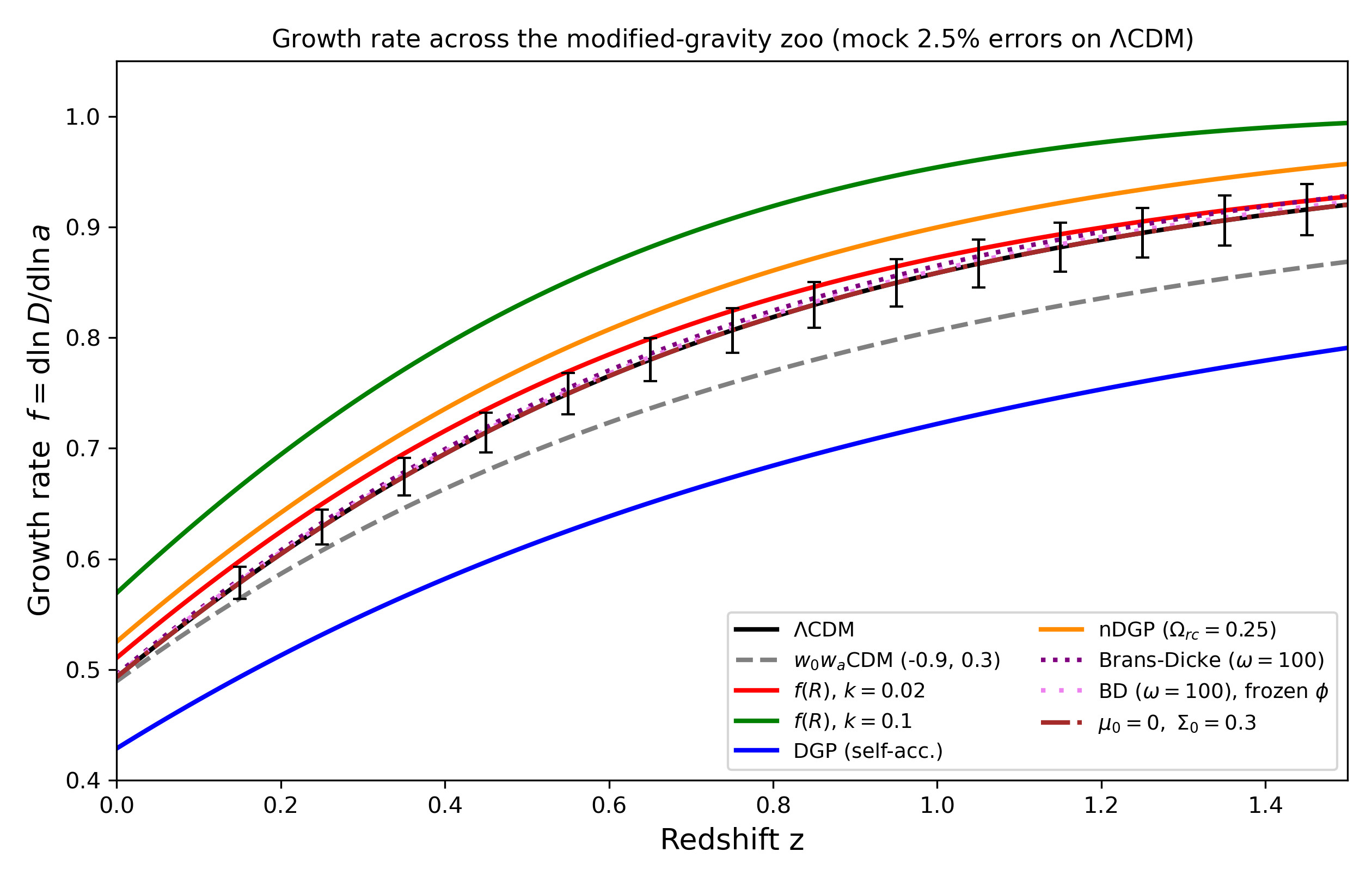
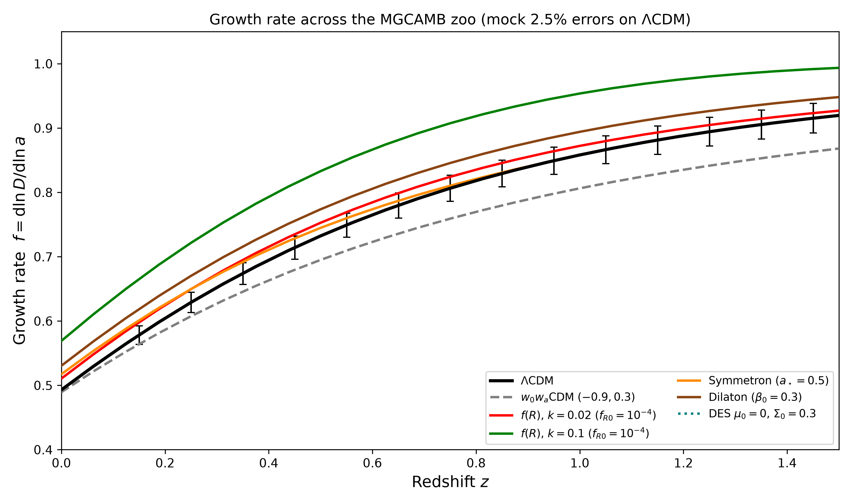
Figure 2: Top: growth rate evolution for different modified gravity models considered in this class. $\mu(a,k)$ has been computed analytically for every model and the growth equation is integrated manually. The whole code is in this notebook. Bottom: Same figure but using the MGCamb code, often used for cosmological studies, computed with this second notebook. Different models are considered but we see a good agreement between analytical predictions and the more refined computation of MGCAMB for models as \(f(R)\). A $2.5\%$ error on $\Lambda$-CDM has been implemented only for illustration, as a precision that could be achieved by future cosmological surveys. For a proper forecast with Euclid, see e.g. Amendola (2016). These plots are inspired from Figure 1 of Ishak et al. (2018), itself a copy of Huterer et al (2015).

Figure 3: $k-z$ dependence of $f$ for the gravity models computed with the MGCAMB notebook. The colorbar shows \(f/f_{\Lambda-\text{CDM}}\). The scale dependence is a direct signature of modified gravity that can not be mimiked by pure dark energy ($w0-wa$ model). Note howver that $w0-wa$ or $\mu_0=0$ models can aquire some $k$ dependence for very large $k$ where the sub-horizon approximation is not valid anymore (to refine)
The only place where the theory of gravity entered our discussion of linear growth was the Poisson equation. Substituting the parametrization introduced above, $\frac{k^2}{a^2}\Psi = -4\pi G\,\mu(a,k)\,\bar\rho_m\Delta_m$, propagates to the source term and to nothing else, one ultimately obtain the modified equation of evolution for the growth rate:
\[\boxed{\;\ddot{\Delta}_m + 2H\dot{\Delta}_m - 4\pi G \mu(k,a)\,\bar\rho_m\,\Delta_m = 0\;}\]Since $\mu$ is precisely the effective Newton constant $G_{\text{eff}}/G$ discussed in the lecture on varying constants, the interpretation is direct: stronger/weaker gravity, faster/slower growth.
Some example of modified gravity model predictions for $f(z)$ are given in Figure 1. We can see that different models have different predictions than $\Lambda$-CDM and that some models predict different shape of this curve for different mode $k$. We see that:
- Growth probes $\mu$, and only $\mu$. $\Sigma$ never appears, because the acceleration of matter never responds to $\Phi$. Conversely, lensing (next section) is blind to $\mu$ at fixed $\Delta_m$. Neither observable alone can fully test gravity: it is their combination — most sharply, their ratio in the $E_G$ statistic that does (defined later). This is clear on Figure 1: models differing only by their value of $\Sigma$ (as $\Lambda$-CDM and DES $\mu_0=0,\Sigma_0=0.3$) are indistinguishable ($\mu_0$ and $\Sigma_0$ are defined later, for now you can just understand them as $\Sigma-1$ and $\mu-1$).
- Scale-dependent growth is itself a signature. If $\mu$ depends on $k$, the factorization $\Delta_m(a,\vec k) = D(a)\Delta_{m,0}(\vec k)$ fails, $D$ becomes $D(a,k)$, and the shape of the matter power spectrum is distorted relative to $\Lambda$CDM. This would be a direct signature of modified gravity, as further illustrated on Figure 3.
On the second point: we see that the Chevalier Polarski Liner (CPL) parametrisation of dark energy $w_0-w_a$ is also added to the plot for illustration (assuming \(w(z) = w_0 + w_a z/(1+z)\) for the dark energy equation of state, $\Lambda$ being \(w_0=-1\) and \(w_a=0\)). This is a pure dark energy model, and no one would generally consider it as modified gravity. However, we see clearly on the figure that such models, while having \(\mu=\sigma=\eta=1\) as in GR modify the growth rate in a way that is totally comparable to modified gravity models. This is coming only from the background modification (\(H(z)\)) in the growth equation. However, there is something that no dark energy model can achieve: the $k$ dependence of the growth rate, as observed in the $f(R)$ model (see Figure 3).
Non-linear growth
Linear theory fails once perturbations become too large ($\Delta_m\sim1$), such that first order (uncoupled) equations stop to be valid. Perturbation theory can be refined to include higher orders but break at some point where the only way out is to rely on heavy $N$ body simulations. As $f$ is increase with the inverse of the scale ($k$), small scales grow quicker. Today we can set the break of the linear regime to $k\gtrsim0.2\,h\,\text{Mpc}^{-1}$, i.e. separations $\lesssim10$ Mpc, but the non-linear scale shrinks with redshift, which is why high-$z$ tracers (Lyman-$\alpha$ forest, quasars) retain linear information down to much smaller separations. Beyond that scale one resorts to N-body simulations — which must now solve the full nonlinear scalar field equations, since this is precisely where screening mechanisms activate (see our later lecture). Signatures are then environment-dependent: unscreened voids and low-mass haloes deviate from GR while massive haloes are screened, motivating probes such as void profiles, marked correlation functions, and cluster splashback radii. We will not discuss in detail here the phenomenology of modified gravity in the non-linear regime. Curious readers can have a look at codes such as hi_cola, which compute $N$-body simulations for Horndeski models.
Galaxy clustering and RSD
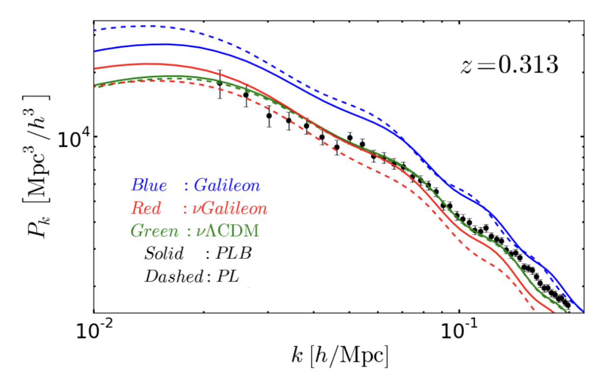
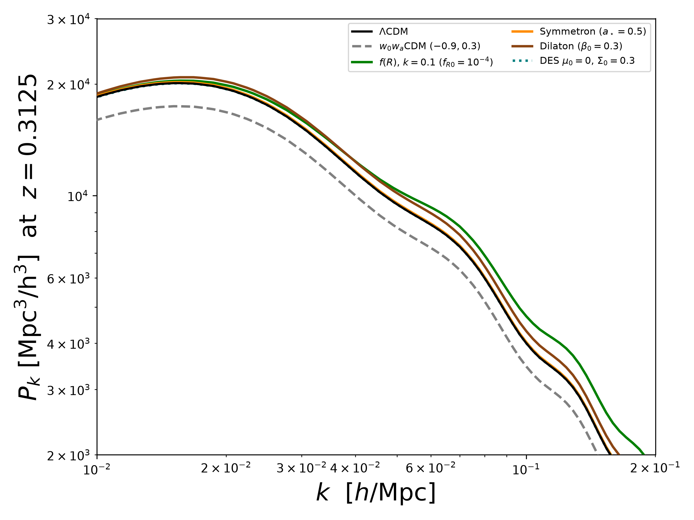
Figure 4: Top: Matter power-spectrum for different Galileon models. From Barreira et al (2014). Bottom: Same figure for our models realised with MGCAMB.
The distortions of $f$ we just derived in a modified gravity theory will in turn modify all cosmological observables related to perturbations, as the matter power-spectrum and all other cosmological observable that quantify structure formation. An illustration of the effect of some modified gravity models on the matter power-spectrum can be found on Figure 4.
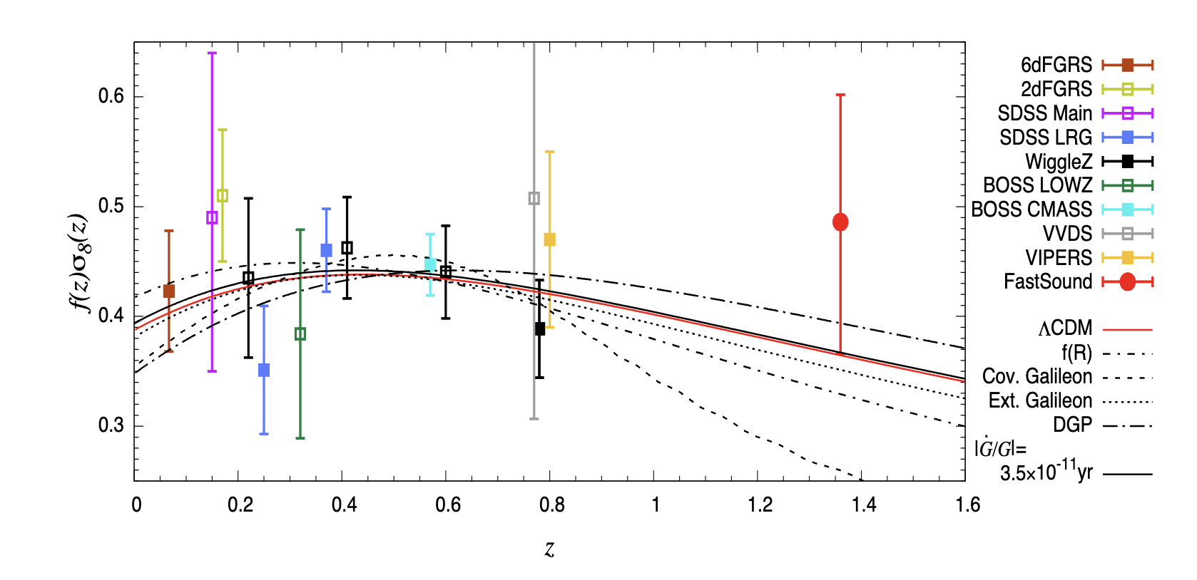
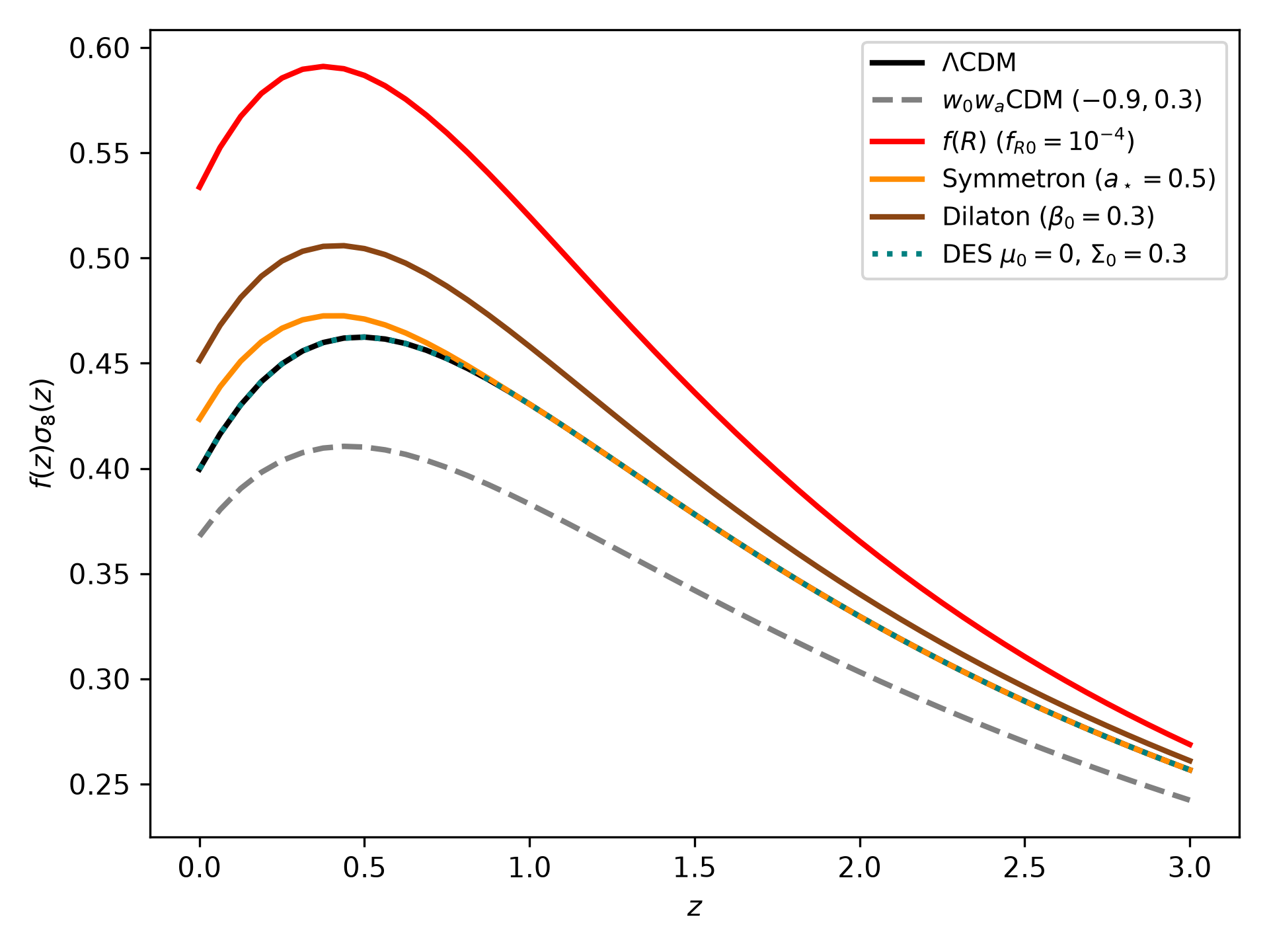
Figure 4: Top: $f(z)\sigma_8(z)$ for different modified gravity models. From Barreira et al (2014). Bottom: Same figure for our models realised with MGCAMB.
However, galaxy surveys targetting the large scale structures of the Universe do not measure $P_m$ or $f$ directly. In practice, one accesses the redshift-space distortions (RSD) due to peculiar velocities of the Galaxies in clusters. Peculiar velocities displace galaxies along the line of sight, squashing the observed clustering anisotropically (Kaiser 1987), and the amplitude of that anisotropy is the combination
\[f\sigma_8(z), \qquad\text{with}\qquad \sigma_8(z) = \sigma_8\,D(z),\]where $\sigma_8$ is the rms linear density fluctuation in spheres of radius $8\,h^{-1}$ Mpc. The combination is used because the unknown galaxy bias $b$ cancels in it, whereas $f$ and $\sigma_8$ are separately degenerate with $b$. This is the quantity reported by DESI, BOSS and eBOSS in the summary table at the end of this lecture. An example of measurements of $f\sigma_8$ confronted with different predictions for modified gravity models can be found on Figure 2. For more on RSD and modified gravity see e.g. Ishak et al. (2018) and references within.
A word on Lymann $\alpha$
Effect on light: Lensing and ISW effect
Weak lensing (cosmic shear)
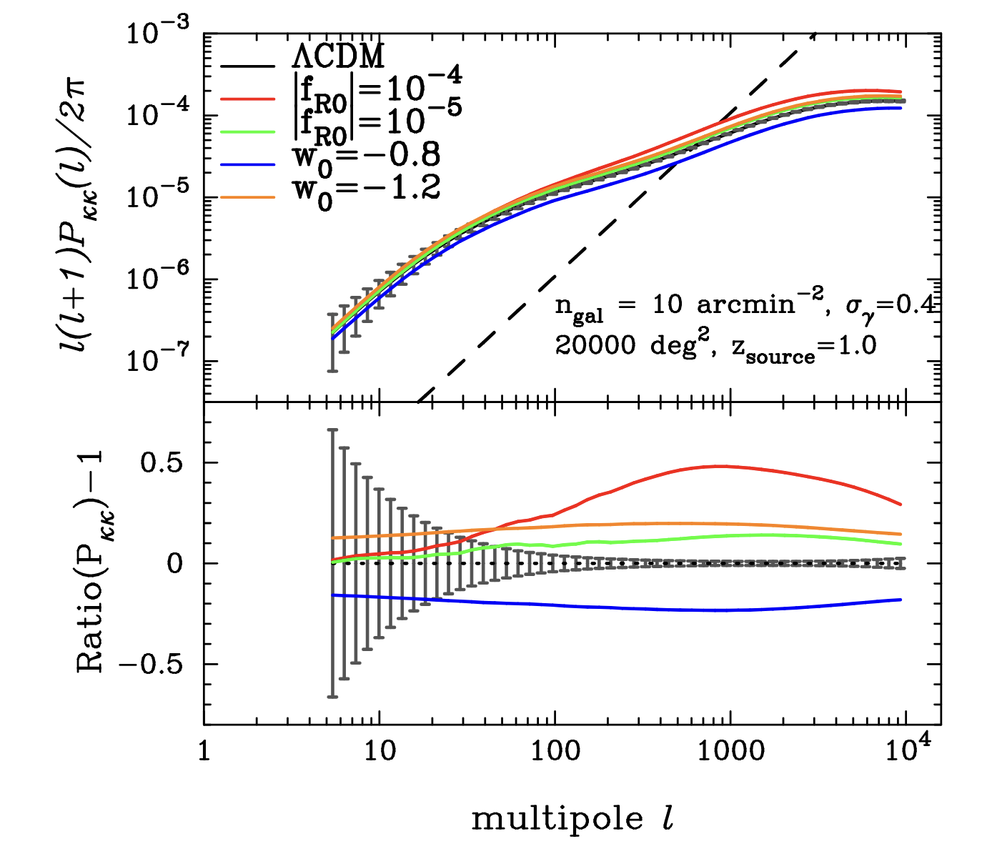
Figure 5: $P_{\kappa\kappa}$ for $\Lambda$-CDM, CPL dark energy models and $f(R)$ models. Error bars are for a survey with sky coverage of 20,000 square degrees with a galaxy density number of 10 per arcminutes squared. Reproduced from figure 2 of Ishak et al. (2018), itself a copy of Shirasaki (2016).
We now turn to the second way to probe modified gravity with cosmology: weighing the same structures with light, in order to isolate the parameter $\Sigma$. We already saw in a previous lecture that light is deflected by point masses in a metric theory of gravity. The deflection angle $\delta \theta$ for a ray coming with impact parameter $b$ can be estimated using the post-Newtonain expansion of General relativity (where $\Psi = \Phi$ naturally), leading to:
\[\delta\theta = \frac{4GM}{c^2 b},\]While we saw that local precision tests could probe sharply this relation in the solar system, it is also tested statically on cosmological scales using at least three different observables: cosmic shear, also called weak lensing (correlated distortions of galaxy shapes), galaxy–galaxy lensing (stacked distortion around foreground galaxies), and CMB lensing (remapping of the CMB by all the structure between us and $z\simeq 1100$). Lensing measures the combination $\Phi+\Psi$ (two times the so-called Weyl potential) sourced by a given $\Delta_m$ — that is, it measures $\Sigma$, exactly as growth measures $\mu$. More precisely, the total deflection angle is proportional to the integral along the line of sight of the gradient of the Weyl potential:
\[\delta \theta \propto \int \vec{\nabla}_\perp(\Phi + \Psi)\text{d}z\]Statistically, in the case of cosmic shear, the lensing is quantified on the sky by the value of two quantities: $\kappa$ the convergence field which quantify the magnification of objects due to lensing and $\gamma$ the complex shear which quantify deformation of circles into ellipses. For a pedagogical introduction to weak lensing, see e.g. Prat (2025). For sources at a single comoving distance $\chi_s$ in a flat universe, $\kappa$ is the line-of-sight integral of the transverse Laplacian of $\Phi_W= (\Phi + \Psi)/2$. Using the Poisson equation above to trade $\Phi_W$ for $\Delta$,
\[\kappa(\hat n) = \int_0^{\chi_s}\!\!\text{d}\chi\;W(\chi)\,\Sigma\big(a(\chi),k\big)\, \Delta(\chi\hat n,\chi), \qquad W(\chi) = \frac{3}{2}\,\Omega_{m,0}\left(\frac{H_0}{c}\right)^{2} \frac{\chi}{a(\chi)}\,\frac{\chi_s-\chi}{\chi_s}.\]Squaring and taking the flat-sky/Limber limit, $k=(\ell+\tfrac12)/\chi$:
\[\boxed{\;P_{\kappa\kappa}(\ell) \;=\;\int_0^{\chi_s}\frac{\text{d}\chi}{\chi^{2}}\; W(\chi)^{2}\;\Sigma^{2}\!\big(a(\chi),k\big)\; P_m\!\left(k=\frac{\ell+\tfrac12}{\chi},\,z(\chi)\right)\;}\]Hence the convergence power-spectrum measured by weak lensing would be sensitive to modified gravity through $\Sigma$ with the $\Sigma^2$ in the above formula, and also through modifications of the matter power spectrum $P_m$ associated to $\mu$. Some example of $P_{\kappa\kappa}$ for various modified gravity models can be found on Figure 5.
The CMB
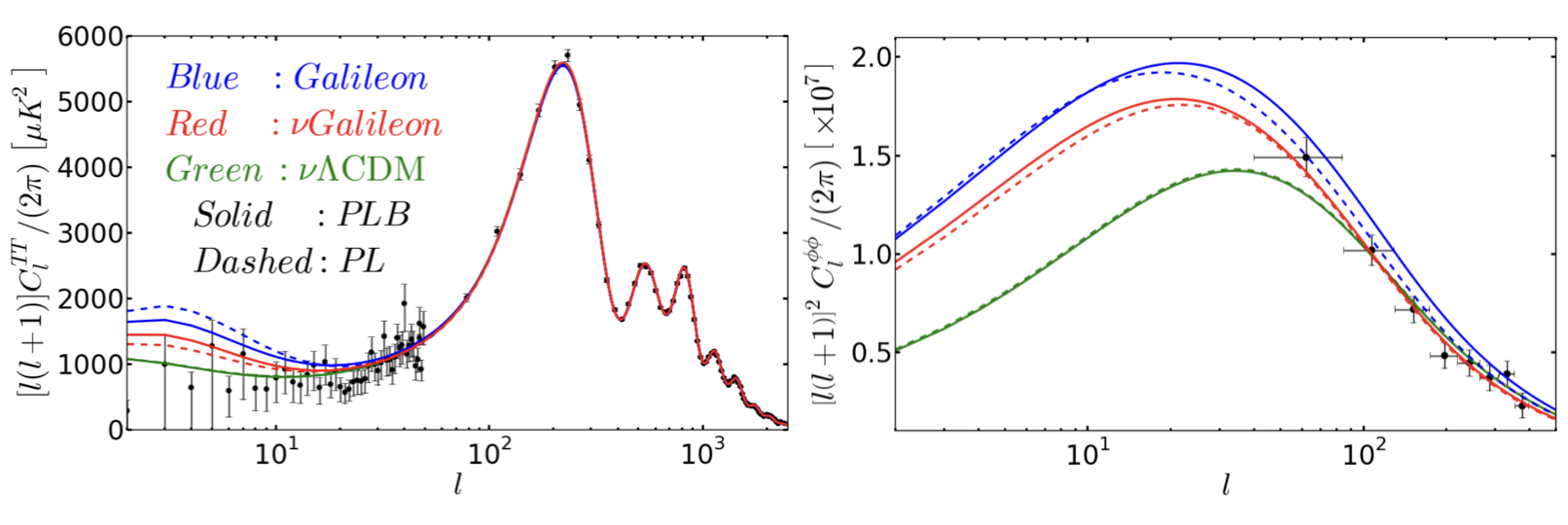
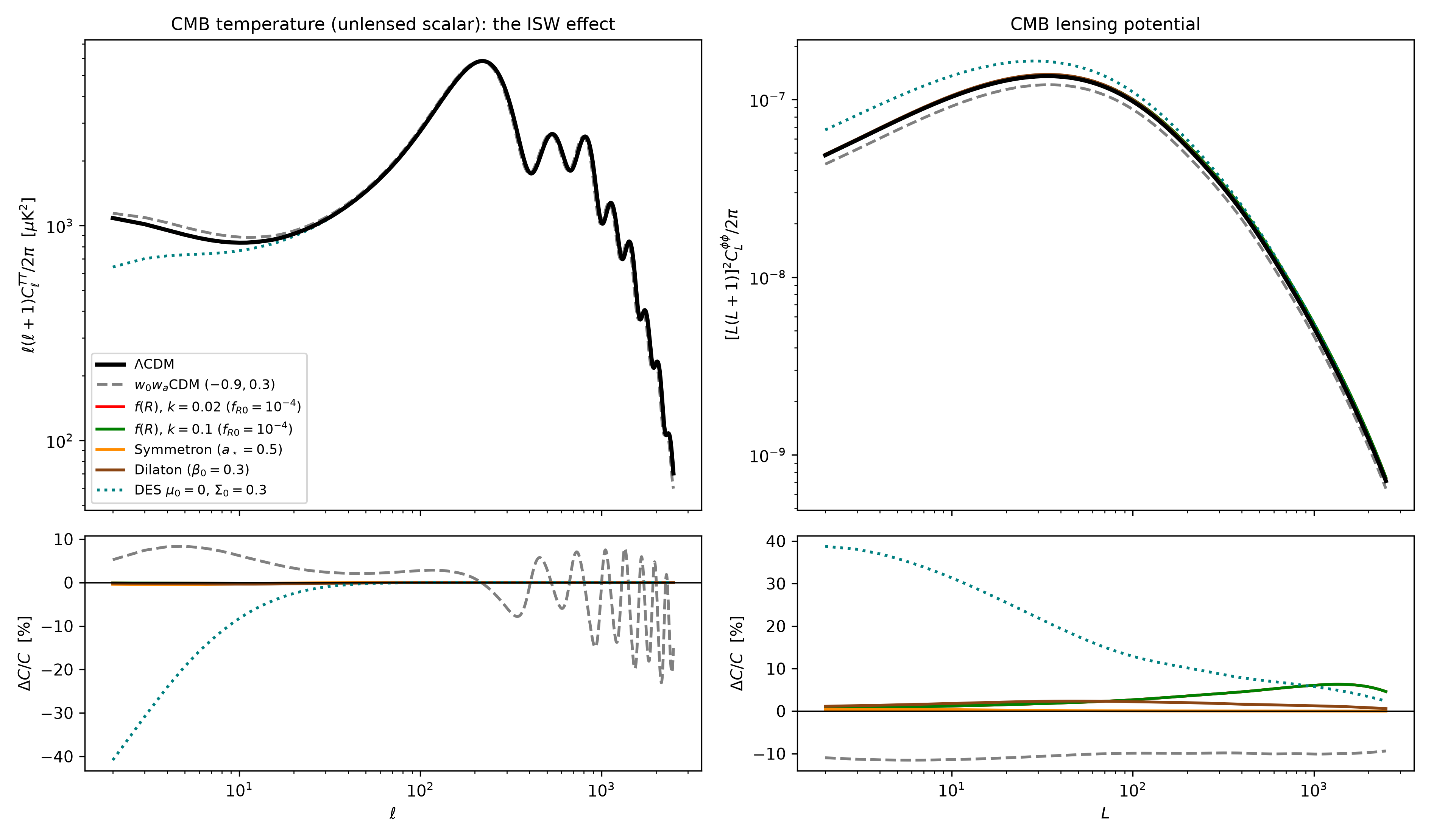
Figure 6: CMB $TT$ and $\phi\phi$ spectra for different modified gravity models: Top: Barreira et al (2014), Bottom: notebook.
The CMB tests gravity from at least three different epochs:
- At $z\simeq 1100$, the acoustic peak structure confirms that the gravitational driving of the photon–baryon fluid in dark matter well follows GR and agrees with a dark matter component (challenging modified gravity theories trying to explain dark matter as a modification of gravity, as explained at the beggining of the class).
- Along the line of sight, the integrated Sachs–Wolfe effect (ISW) generates temperature anisotropies whenever the potentials evolve. Indeed, photons gain some energy when entering a potential well and loose it when going out. If potential evolve during this travelling time, the photons will end up with more or less energy (frequency shift) than when they entered the well (if the well decays or get sharper respectively). This energy change impacts the photon spectrum in a fashion proportional to the integral of the time evolution of the Weyl potential as $\Delta T/T \propto \int (\dot\Phi+\dot\Psi)\,\text{d}t$. CMB photons are emitted after radiation domination (recombination occurs at $z\simeq 1100$, while matter radiation equality is at $z\simeq 3500$), and they travel through matter and dark energy domination era to reach us. From the growth equation, one can infer the potentials are constant in a matter-dominated — so ISW detection (via cross-correlation with galaxy surveys) directly probes the decay of $\Phi+\Psi$ induced by dark energy or by modified gravity.
- The, CMB lensing smooths the acoustic peaks and rotates the CMB polarisation (transforms $E$-modes into $B$-modes). It is now measured at $>40\sigma$, anchoring the amplitude of the Weyl potential integrated to high redshift. Comparing the lensing amplitude with the one predicted from the primary CMB is a stringent internal consistency test of GR: ACT DR6 finds $A_{\text{lens}}=1.013\pm0.023$ with respect to the Planck $\Lambda$CDM prediction (Qu et al. 2024), i.e. agreement at the $2\%$ level over a $\sim1100$-fold range in redshift. As for ISW, CMB lensing can be cross-correlated with Galaxy surveys to obtain an even more powerful constraining power.
CMB $TT$ and $\phi\phi$ spectra are displayed on Figure 6 for different modified gravity models. We see that models with the stronger impact on the spectra are the ones in which $\Sigma\neq1$.
While almost all possible information has been extracted out of the CMB temperature (cosmic variance limited), contemporary research focuses on the measurement of the polarisation of the CMB. The primordial polarisation spectra are not impacted by the ISW effect and are thus insensitive to the value of $\Sigma$. However, refined polarisation measurements allow a better characterisation of the lensing and are sensitive to parity and Lorentz violating signals like cosmic birefringence, in direct violation with the EEP and possibly induced by axion like particles coupled to the photons. Furthermore, future high precision measurements of possible deviation to the CMB blackbody SED, the spectral distortions could shed light on new fields partaking to gravity which could have injected energy in the early universe.
The $E_G$ statistic: weighing the same structures with light and with matter
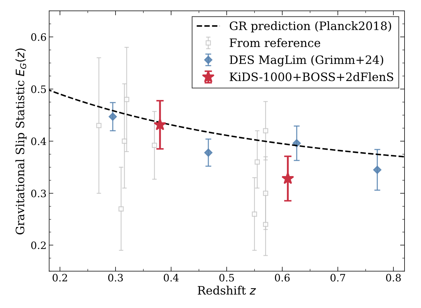
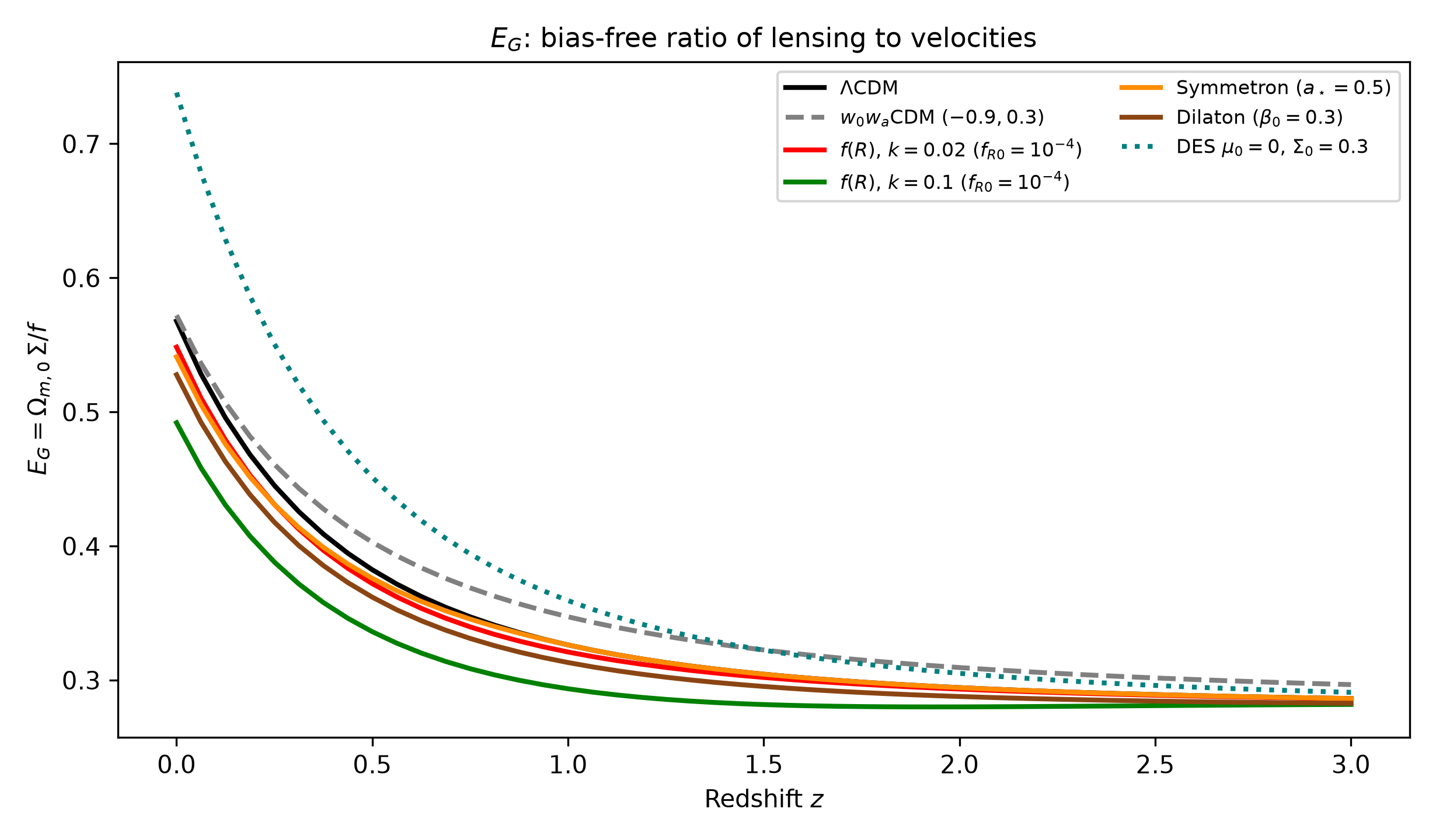
Figure 7: Top: some measurements of the $E_G$ statistics from Zhang (2026). Right: value of $E_G$ for different modified gravity models from the tutorial notebook
There exist multiple ways to parametrize cosmological modification of gravity and we will not review them all here. We already saw the $\mu/\Sigma,\eta$ parametrisation as well as the growth index $\gamma$. Another powerful quantity to measure is the so-called $E_G$ statistics, defined as:
\[E_G(k,z)= \frac{k^2 (\Psi + \Phi)}{3H_0^2 a^{-1}f \delta_m}\]In other word: $E_G$ looks at the ratio of lensing over growth. Here again, the possible scale dependence of $E_G$ would be a direct signature of modified gravity, as in GR, there is no $k$ dependence:
\[E_G(z) = \frac{\Omega_m(z)}{f(z)}\]The value of $E_G$ for different modified gravity models can be found in Figure 7. We see that, contrarily to other probes, $E_G$ is able to discriminate between GR and any other modified gravity models (independently of whether or not it impact only growth or only lensing).
Constraints on the $\mu$, $\Sigma$, $\eta$ parametrization
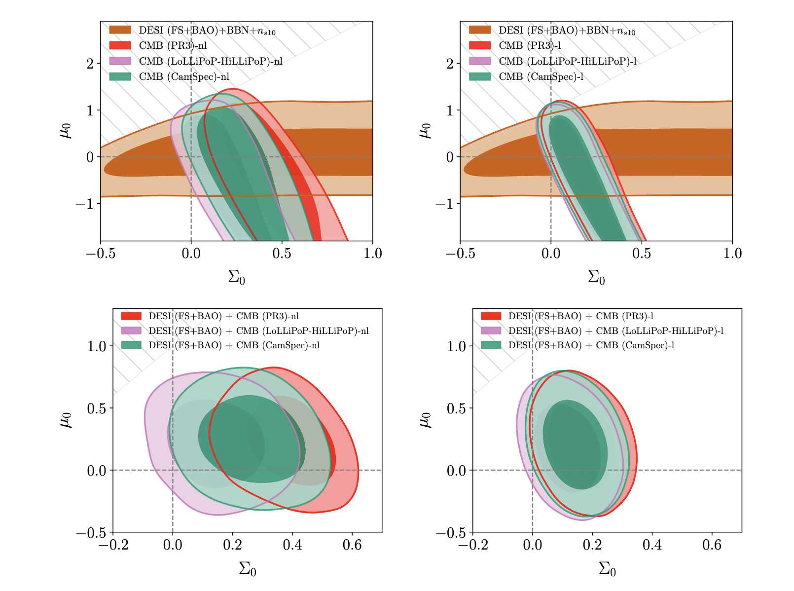
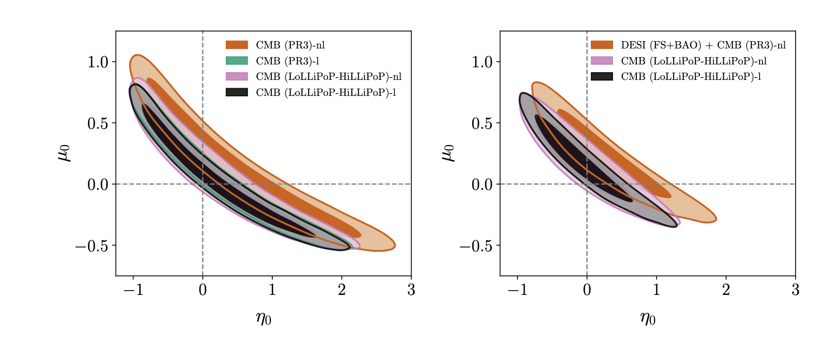
Figure 8: constraints on the $\mu_0-\Sigma_0-\eta_0$ parametrization using different cosmological data-set. From DESI (2025).
The following table gathers the logic of this lecture in one place. A warning before reading it: the numbers are not directly comparable to one another. Each collaboration adopts its own time dependence for $\mu$ and $\Sigma$, its own scale cuts, and its own external datasets. In the above figures:
\[\boxed{\;\mu(a,k) = 1 + \mu_0\,\frac{\Omega_{\rm DE}(a)}{\Omega_\Lambda} \left[\frac{1 + c_1\left(\lambda H(a)/k\right)^2}{1 + \left(\lambda H(a)/k\right)^2}\right]\;}\] \[\boxed{\;\Sigma(a,k) = 1 + \Sigma_0\,\frac{\Omega_{\rm DE}(a)}{\Omega_\Lambda} \left[\frac{1 + c_2\left(\lambda H(a)/k\right)^2}{1 + \left(\lambda H(a)/k\right)^2}\right]\;}\]with $\Omega_{\rm DE}(a)$ the dark-energy density parameter, $\Omega_\Lambda$ its value today, and $\lambda$ a dimensionless constant setting the transition wavenumber $k_\star = \lambda H(a)$.
- Time dependence — the prefactor $\Omega_{\rm DE}(a)/\Omega_\Lambda$ switches the modification off whenever dark energy is subdominant, so gravity is GR throughout matter domination and the CMB is untouched.
- Scale dependence — writing $x = (\lambda H/k)^2$, the bracket is $(1+c_1x)/(1+x)$, which interpolates between two constants: it tends to $1$ for $k \gg \lambda H$ (small scales) and to $c_1$ for $k \ll \lambda H$ (near-horizon scales).
- Hence $\mu_0$ and $\Sigma_0$ are the present-day, small-scale amplitudes: at $a=1$ and $k\gg\lambda H$ one has $\mu \to 1+\mu_0$ and $\Sigma \to 1+\Sigma_0$.
Quoting “the” constraint on $\mu_0$ without specifying the parametrization is meaningless — this is the main practical difference with the PPN parameters, which are defined unambiguously. Take the table as an order-of-magnitude map, not as a leaderboard.
| Observable | Potential(s) probed | Parameter | Regime | Example dataset | Representative constraint | Next (forecast) |
|---|---|---|---|---|---|---|
| RSD / peculiar velocities | $\Psi$ | $\mu$ | linear, $z\lesssim 2$ | DESI DR1 full-shape + CMB + SN | $\mu_0 = 0.05\pm0.22$ — Ishak et al. (2024) | DESI (5-yr), Euclid spectroscopic ($0.9<z<1.8$), Subaru PFS, Roman; $f\sigma_8$ to $\sim1\%$ per bin, $\sigma(\mu_0)$ improved by $\sim$10× |
| Growth index (RSD + CMB + WL) | $\Psi$ | $\mu$ (via $\gamma_g$) | linear, $z\lesssim 2$ | Planck + $f\sigma_8$ + WL + peculiar velocities | $\gamma_g = 0.633^{+0.025}_{-0.024}$ vs $6/11\simeq0.545$ in GR ($3.7\sigma$) — Nguyen et al. (2023) | Euclid + DESI + Rubin/LSST; $\sigma(\gamma_g)\sim$ few $\times10^{-3}$ — enough to settle the current $3.7\sigma$ either way |
| Cosmic shear + galaxy clustering ($3\times2$pt) | $\Phi+\Psi$ | $\Sigma$ | (quasi-)linear | DES Y3 $3\times2$pt alone | $\Sigma_0 = 0.6^{+0.4}_{-0.5}$ — DES Collaboration (2023) | Euclid (DR1 images end 2026, cosmology 2027), Rubin/LSST (10-yr), Roman high-latitude survey |
| $3\times2$pt + CMB + SN | $\Phi+\Psi$, $\Psi$ | $\Sigma$, $\mu$ | (quasi-)linear | DES Y3 + external | $(\Sigma_0,\mu_0) = (0.04\pm0.05,\;0.08^{+0.21}_{-0.19})$ — DES Collaboration (2023); $\Sigma_0=0.008\pm0.045$ — DESI (2024) | Euclid $\times$ Simons Observatory: $\sigma(\Sigma_0)\sim10^{-2}$, up to two orders of magnitude beyond Planck alone for some models — Euclid Collaboration (2025) |
| CMB lensing | $\Phi+\Psi$ | $\Sigma$ | linear, $0.5\lesssim z\lesssim 5$ | ACT DR6 ($43\sigma$, 2.3% precision) | $A_{\text{lens}} = 1.013\pm0.023$ — Qu et al. (2024) | Simons Observatory ($\sim$sub-percent on the lensing amplitude), CMB-S4 if funded; decisive for the $\Sigma_0$ claim of Du et al. (2026) |
| ISW (cross-correlation) | $\dot\Phi+\dot\Psi$ | $\Sigma$ (time evol.) | ultra-large scales | Planck × NVSS, SDSS, WISE, CMB lensing | detection at $\simeq4\sigma$, amplitude consistent with $\Lambda$CDM — Planck 2015 XXI | SO / CMB-S4 $\times$ Euclid / Rubin; $\sim7$–$8\sigma$, but cosmic-variance limited — the one entry that cannot improve indefinitely |
| $E_G$ | ratio lensing/velocity | $\Sigma/\mu$ | linear, $0.2<z<0.7$ | KiDS-1000 × BOSS + 2dFLenS | 15–20% per bin, GR-consistent with $\Omega_m=0.27\pm0.04$ — Blake et al. (2020) | Euclid $\times$ DESI, Rubin $\times$ DESI; few-% per bin, turning $E_G$ from a consistency check into a real measurement |
| BBN / CMB peaks | background $H$ | $G_{\text{eff}}/G$ | $z\gtrsim10^3$ | light-element abundances, CMB peak positions | $\lvert G_{\text{eff}}/G - 1\rvert \lesssim 0.05$–$0.1$ (see the previous lecture) | SO, CMB-S4; modest gains — this row is limited by BBN nuclear rates, not by CMB precision |
Summary table: which observable probes what.
Further reading/watching
- Dodelson & Schmidt, Modern Cosmology, 2nd ed., Academic Press (2020).
- Baumann, Cosmology, Cambridge University Press (2022); free lecture-note version.
- Amendola & Tsujikawa, Dark Energy: Theory and Observations, Cambridge University Press (2010).
- Modified Gravity 2: Phenomenology — Bhuvnesh Jain
- Ishak, Testing general relativity in cosmology, Living Rev. Relativ. 22, 1 (2019).
- Ferreira, Cosmological tests of gravity, Ann. Rev. Astron. Astrophys. 57, 335 (2019).
- Amendola et al. (Euclid Theory WG), Cosmology and fundamental physics with the Euclid satellite, Living Rev. Relativ. 21, 2 (2018).
- Ma & Bertschinger, Cosmological perturbation theory in the synchronous and conformal Newtonian gauges, Astrophys. J. 455, 7 (1995).