Horndeski theories

Overview: additional degrees of freedom

In the previous class, we discussed how to add a scalar field to curved space-time, and how such an addition allows us to go beyond general relativity — with the historical example of Brans-Dicke theory. But the landscape of possibilities is enormous. Lovelock’s theorem tells us that one of the options to go beyond GR is to add a new degree of freedom but it does not tell us which and how. One may add one or several scalar, vector or tensor fields on top of GR, in any combination, and an illustration of the most common such ideas is displayed in Figure 1. Covering them all in detail is simply impossible.

Among them, a few seem to us especially natural, because they introduce no new external field at all: instead of adding something to GR, they release a structure that GR had frozen by hand. Allowing a non-vanishing torsion breaks our axiom (S3b); giving a mass to the graviton relaxes the assumption that it propagates exactly at the speed of light. We will discuss both in the coming lectures.

In the present class we focus on the Horndeski framework (Horndeski 1974), rediscovered four decades later under the name of generalised galileons (Deffayet et al. 2011). It is the most general theory one can build in four dimensions from the metric and a single scalar field, whose equations of motion remain of second order. That last requirement is not an aesthetic preference. By Ostrogradsky’s theorem, a non-degenerate Lagrangian containing derivatives higher than second order propagates a ghost: a degree of freedom whose energy is unbounded from below, which makes the vacuum unstable to the spontaneous creation of ghost–ordinary particle pairs. Second-order field equations are therefore not elegance, they are survival. Horndeski’s achievement was to show that this demand closes the problem: the answer is a finite list, parametrised by four free functions of the scalar field and its kinetic term, which contains every healthy scalar-tensor theory. Quintessence and Brans-Dicke both sit inside it as particular choices of these functions. Instead of examining models one at a time, we can therefore treat the entire class at once — which is precisely why the framework is so useful.

Such models are extensively studied by cosmologists and are of course deeply intertwined with the question of dark energy. Since our focus here is modified gravity, the ability of a model to reproduce today’s cosmic acceleration will not be our primary criterion, though it is obviously a desirable feature. One might then be tempted to restrict attention to models that genuinely modify the Einstein-Hilbert term, as opposed to those that merely add a new matter component. But as we saw when confronting quintessence with Brans-Dicke, that distinction is not frame-invariant: a conformal transformation moves a non-minimal coupling out of the gravitational sector and into the matter one, and back again. “Modified gravity” and “new matter” are, to a large extent, two descriptions of the same physics — and one should be suspicious of any claim that depends on which of the two labels one has chosen.

In this class, the presentation of Horndeski theory is inspired by the great lectures of Tessa Baker and her associated lecture notes in which you will find the detail of each equation. See also Bellini & Sawicki 2014 for the detailed derivations.

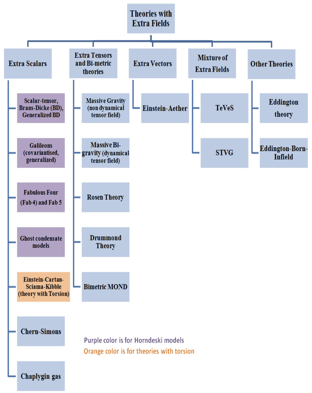
Figure 1: A roadmap of some additional field models of modified gravity. Credit: Ishak et al. (2024).

Horndeski theory

We write $\phi_\mu \equiv \nabla_\mu\phi$. The kinetic scalar is $X \;\equiv\; -\tfrac12\,\nabla^\mu\phi\,\nabla_\mu\phi ,$ so that for a homogeneous cosmological field $X = \tfrac12\dot\phi^2 \ge 0$. Horndeski’s theorem (1974): the most general Lagrangian built from $g_{\mu\nu}$ and a single scalar $\phi$ in 4D whose Euler–Lagrange equations are at most second order in derivatives (hence free of Ostrogradsky ghosts) is $\mathcal{L}_{\rm H}=\sum_{i=2}^{5}\mathcal{L}_i$ with

\[S_{\rm H} = \int d^4x\,\sqrt{-g}\;\big(\mathcal{L}_2+\mathcal{L}_3+\mathcal{L}_4+\mathcal{L}_5\big) + S_m[g_{\mu\nu},\psi_m]\] \[\boxed{ \begin{aligned} \mathcal{L}_2 &= G_2(\phi,X) \\[4pt] \mathcal{L}_3 &= -\,G_3(\phi,X)\,\Box\phi \\[4pt] \mathcal{L}_4 &= G_4(\phi,X)\,R \;+\; \frac{\text{d}G_{4}}{\text{d}X}\Big[(\Box\phi)^2 - \nabla_\mu\nabla_\nu\phi\,\nabla^\mu\nabla^\nu\phi\Big] \\[4pt] \mathcal{L}_5 &= G_5(\phi,X)\,G_{\mu\nu}\nabla^\mu\nabla^\nu\phi \;-\; \frac{1}{6}\,\frac{\text{d}G_{5}}{\text{d}X}\Big[(\Box\phi)^3 - 3\,\Box\phi\,\nabla_\mu\nabla_\nu\phi\,\nabla^\mu\nabla^\nu\phi + 2(\nabla_\mu\nabla_\nu\phi\,\nabla^\nu\nabla^\rho\phi\,\nabla_\rho\nabla^\mu\phi)\Big] \end{aligned}}\]

A few comments facing these Lagrangians:

$G_2, G_3, G_4, G_5$ are four arbitrary functions of $(\phi, X)$.
$G_2$ is also often written $K$, is the kinetic term of the scalar field. Note however that this name can generate confusion, as any simple potentials like a mass term $V=m^2\phi^2/2$ would also be contained in $G_2$.
$G_3$ is related to possible screening, as Vainshtein screening. We will rediscuss it in more details in our dedicated lecture.
$G_4$ contains coupling and modifications to the gravity sector. GR is solely contained within the $\mathcal{L}_4$ term, with $G_4(\phi,X)=1/(16\pi G)$.
$G_5$ contains complex derivative couplings between gravity and the field and highly non linear field dynamics.

Note that the non-minimal terms $\propto \text{d} G_{4}/\text{d}X$ and $\text{d} G_{5}/\text{d}X$ are counterterms: they are not optional. Their precise coefficients cancel the higher-derivative pieces generated by varying $G_4 R$ and $G_5 G_{\mu\nu}\nabla\nabla\phi$, keeping the field equations second order. Change a coefficient and you reintroduce a ghost. Note also that matter is coupled to $g_{\mu\nu}$ alone, exactly as in the Jordan frame of Brans-Dicke. Horndeski theories are therefore metric theories: they satisfy the WEP and the EEP by construction, and violate the SEP. Everything we said about frames in the previous class applies unchanged. As an historical note: Horndeski’s original 1974 paper was written in a different (equivalent) parametrization and was largely forgotten; the form above emerged from the Galileon programme (Nicolis, Rattazzi & Trincherini 2009) and its covariantization (Deffayet, Esposito-Farèse & Vikman 2009), then Deffayet et al. proved the equivalence.

Now, the powerful advantage of this framework is that it allows to rewrite and study all at once virtually all possible scalar tensor theories one can come up with. Quintessence and Brans-Dicke are both a subset of Horndeski theories as well as many others as illustrated in the following table:

Theory	$G_2$	$G_3$	$G_4$	$G_5$
GR	$0$	$0$	$M_{\rm Pl}^2/2$	$0$
GR + $\Lambda$	$-M_{\rm Pl}^2\Lambda$	$0$	$M_{\rm Pl}^2/2$	$0$
Quintessence	$X - V(\phi)$	$0$	$M_{\rm Pl}^2/2$	$0$
Brans–Dicke	$2\omega X/\phi$	$0$	$\phi/16\pi$	$0$
k-essence	$G_2(\phi,X)$	$0$	$M_{\rm Pl}^2/2$	$0$
$f(R)$	$-\tfrac{M_{\rm Pl}^2}{2}\big(\phi f’(\phi)-f(\phi)\big)$	$0$	$\tfrac{M_{\rm Pl}^2}{2}f’(\phi)$	$0$
Kinetic gravity braiding	$G_2(\phi,X)$	$G_3(\phi,X)$	$M_{\rm Pl}^2/2$	$0$
Cubic Galileon	$X$	$c_3 X$	$M_{\rm Pl}^2/2$	$0$
Non-minimal $\xi\phi^2 R$	$X-V$	$0$	$\tfrac12(M_{\rm Pl}^2+\xi\phi^2)$	$0$
Gauss–Bonnet $\xi(\phi)\mathcal{G}$	$8\,\xi^{(4)}X^2(3-\ln X)$	$4\,\xi^{(3)}X(7-3\ln X)$	$4\,\xi^{(2)}X(2-\ln X)$	$-4\,\xi^{(1)}\ln X$

Where we introduce normalisation by the Planck mass: $M_{\rm Pl}^2= 1/(8\pi G)$, which is a familiar convention for particle physicists. Now we could roughly consider that modified gravity theories, as Brans-Dicke or $f(R)$, are the one where the field appears into the $G_4$ term. Dark energy models would be the ones with $G_4= M_{\rm Pl}^2/2$ and $G_5=0$ (as $G_5$ couples to the Einstein tensor). This would for example be the case of quintessence and $k$-essence. However, as we already discussed in regard of the Einstein/Jordan frames, this is partly arbitrary an distinction.

If you have already some knowledge on modified gravity, you may be surprised to see a theory as $f(R)$ in this table, which is a well known theory that goes around lovelock theorem by adding higher orders to the gravity Lagrangian: looks like a modification of the geometry, but it is nothing more than one extra scalar in disguise.

The Horndeski alphas

The key simplification is that at the level of linear perturbations on a cosmological background, all of Horndeski is captured by four functions of time alone (Bellini & Sawicki 2014):

function	name	meaning
$\alpha_M\equiv \nu_T-3$	Planck-mass run rate	rate of change of the effective gravitational constant or Planck mass, related to the friction $\nu_T$ of gravitational waves.
$\alpha_T \equiv c_T^2-1$	tensor speed excess	gravitational waves travel at $c_T\neq c$
$\alpha_B$	braiding	kinetic mixing between the scalar and the metric; makes dark energy cluster
$\alpha_K$	kineticity	the scalar’s own kinetic energy; controls its sound speed

In GR, these four coefficients are strictly zero and in perturbation theory all the deviations from GR can be quantified by these $\alpha_i$. In practice then, these are the coefficients we can hope to constraint observationally. Formally, these have the following (awful) expressions in terms of the functions $G_i$ and their derivatives:

\[\begin{aligned} M_*^2 \;=\;& 2\left(G_4 - 2X\frac{\text{d}G_4}{\text{d}X} + X\frac{\text{d}G_5}{\text{d}\phi} - XH\frac{\text{d}\phi}{\text{d}t}\frac{\text{d}G_5}{\text{d}X}\right) \\[10pt] \alpha_M \;\equiv\;& \frac{\text{d}\ln M_*^2}{\text{d}\ln a} \\[4pt] \;=\;& \frac{2}{M_*^2}\Bigg[\,2X\left(\frac{\text{d}G_4}{\text{d}X} - \frac{\text{d}G_5}{\text{d}\phi} + 2X\left(\frac{\text{d}^2G_4}{\text{d}X^2} - \frac{\text{d}^2G_5}{\text{d}X\,\text{d}\phi}\right)\right) \\ &+ \frac{1}{H}\frac{\text{d}\phi}{\text{d}t}\left(\frac{\text{d}G_4}{\text{d}\phi} - X\left(2\frac{\text{d}^2G_4}{\text{d}X\,\text{d}\phi} - \frac{\text{d}^2G_5}{\text{d}\phi^2}\right)\right) + XH\frac{\text{d}\phi}{\text{d}t}\left(3\frac{\text{d}G_5}{\text{d}X} + 2X\frac{\text{d}^2G_5}{\text{d}X^2}\right) \\ &- \frac{X}{H}\frac{\text{d}G_5}{\text{d}X}\frac{\text{d}H}{\text{d}t}\frac{\text{d}\phi}{\text{d}t} \\ &- \left(3X\frac{\text{d}G_5}{\text{d}X} + 2X^2\frac{\text{d}^2G_5}{\text{d}X^2} + \frac{1}{H}\frac{\text{d}\phi}{\text{d}t}\left(\frac{\text{d}G_4}{\text{d}X} - \frac{\text{d}G_5}{\text{d}\phi} + X\left(2\frac{\text{d}^2G_4}{\text{d}X^2} - \frac{\text{d}^2G_5}{\text{d}X\,\text{d}\phi}\right)\right)\right)\left(\frac{\text{d}^2\phi}{\text{d}t^2} + H\frac{\text{d}\phi}{\text{d}t}\right)\Bigg] \\[10pt] \alpha_K \;=\;& \frac{2X}{H^2M_*^2}\Bigg[\,\frac{\text{d}G_2}{\text{d}X} - 2\frac{\text{d}G_3}{\text{d}\phi} + 2X\left(\frac{\text{d}^2G_2}{\text{d}X^2} - \frac{\text{d}^2G_3}{\text{d}X\,\text{d}\phi}\right) \\ &+ 6H\frac{\text{d}\phi}{\text{d}t}\left(\frac{\text{d}G_3}{\text{d}X} - 3\frac{\text{d}^2G_4}{\text{d}X\,\text{d}\phi} + X\left(\frac{\text{d}^2G_3}{\text{d}X^2} - 2\frac{\text{d}^3G_4}{\text{d}X^2\,\text{d}\phi}\right)\right) \\ &+ 6H^2\left(\frac{\text{d}G_4}{\text{d}X} - \frac{\text{d}G_5}{\text{d}\phi} + X\left(8\frac{\text{d}^2G_4}{\text{d}X^2} - 5\frac{\text{d}^2G_5}{\text{d}X\,\text{d}\phi}\right) + 2X^2\left(2\frac{\text{d}^3G_4}{\text{d}X^3} - \frac{\text{d}^3G_5}{\text{d}X^2\,\text{d}\phi}\right)\right) \\ &+ 2H^3\frac{\text{d}\phi}{\text{d}t}\left(3\frac{\text{d}G_5}{\text{d}X} + 7X\frac{\text{d}^2G_5}{\text{d}X^2} + 2X^2\frac{\text{d}^3G_5}{\text{d}X^3}\right)\Bigg] \\[10pt] \alpha_B \;=\;& \frac{2}{HM_*^2}\frac{\text{d}\phi}{\text{d}t}\Bigg[\,-\frac{\text{d}G_4}{\text{d}\phi} + X\left(\frac{\text{d}G_3}{\text{d}X} - 2\frac{\text{d}^2G_4}{\text{d}X\,\text{d}\phi}\right) \\ &+ 2H\frac{\text{d}\phi}{\text{d}t}\left(\frac{\text{d}G_4}{\text{d}X} - \frac{\text{d}G_5}{\text{d}\phi} + X\left(2\frac{\text{d}^2G_4}{\text{d}X^2} - \frac{\text{d}^2G_5}{\text{d}X\,\text{d}\phi}\right)\right) + XH^2\left(3\frac{\text{d}G_5}{\text{d}X} + 2X\frac{\text{d}^2G_5}{\text{d}X^2}\right)\Bigg] \\[10pt] \alpha_T \;\equiv\;& c_T^2 - 1 \;=\; \frac{2X}{M_*^2}\left[\,2\frac{\text{d}G_4}{\text{d}X} - 2\frac{\text{d}G_5}{\text{d}\phi} - \left(\frac{\text{d}^2\phi}{\text{d}t^2} - H\frac{\text{d}\phi}{\text{d}t}\right)\frac{\text{d}G_5}{\text{d}X}\right] \\[10pt] \end{aligned}\]

Again, see Bellini & Sawicki 2014. Just like for $\mu$, $\Sigma$ and $\eta$ it is common to constraint some specific parametrisation of the Hordneski parameters. The standard parametrisation is to assume that the field is anyhow responsible for some form of evolving dark energy. Then one consider:

\[\alpha_M(z) = c_M \frac{\Omega_\Lambda(z)}{\Omega_{\Lambda_0}}\] \[\alpha_B(z) = c_B \frac{\Omega_\Lambda(z)}{\Omega_{\Lambda_0}}\]

In practice, it is much easier to constrain $c_M$ and $c_B$ than $\alpha_M$ and $\alpha_B$ as will be discussed below.

The GW170817 constraint and Luminal Horndeski theory

It is possible to show that in the case of Horndeski theory, the propagation of a gravitational wave is given by:

\[\boxed{\;\ddot{h}_{ij} \;+\; \big(3+\alpha_M\big)\,H\,\dot{h}_{ij} \;+\; \big(1+\alpha_T\big)\,\frac{k^2}{a^2}\,h_{ij} \;=\; 0\;}\]

This computation requires to derive all the perturbation equation for tensor modes and is rather lengthy, so we will just admit this result here. We see that, in Hordneski theory, the graviton remains massless. Deviation from GR are driven entirely by $\alpha_T$ and $\alpha_M$ and thus by the functions $G_{4X}$ and $G_5$.

The measurements from GW170817 + GRB 170817A discussed in the dedicated lecture, allows to drastically constrain the functions $\alpha_T$ and $\alpha_M$ here. The constraints on the speed of gravitational waves $c_T$, immediately translate to:

\[\vert \alpha_T \vert \lesssim 10^{-15}\]

Rederiving the bound on $\alpha_T$

Inspired by the lecture of T. Baker (2025), we can easily re-obtain the constraint on the speed of gravitational waves from GW170817 simply knowing that the time delay between photons and the gravitational waves was observed to be $\Delta t= 1.7$ s, and that their distance is estimated to be $d\sim 40$ Mpc. Indeed, as this distance is very close in term of cosmology, we can simply assume that velocity is the distance divided by the time elapsed and thus:

\[\begin{align} \Delta t &= t_\gamma - t_{GW} \\ &= \frac{d}{c_\gamma} - \frac{d}{c_T}\\ &= d(1 - \frac{1}{\sqrt{1+\alpha_T}})\\ &\simeq d \left(1-1 + \frac{\alpha_T}{2}\right)\\ & \alpha_T \simeq \frac{2c_\gamma \Delta t}{d} \end{align}\]

Plugging in the numbers, one finds easily $\vert \alpha_T \vert \lesssim 10^{-15}$.

$\alpha_M$ itself is poorly constrained by gravitational waves, as discussed in the dedicated lecture, because of the poor measurement of $\Xi_0$. Using dark sirens and assuming the $c_M$ parametrisation above, one can reach $c_M = 1.5^{+2.2}_{-2.1}$ (see Fig. 9 of Chen et al (2023)). However, it is expected to improve drastically with future gravitational wave surveys.

Now, this cancellation of $\alpha_T$ leads to a drastic simplification of the Horndeski Lagrangian (see proof box below). The surviving Horndeski class simplifies drastically to the so-called luminal Hordneski Lagrangian

\[\boxed{\mathcal{L} = G_2(\phi,X) - G_3(\phi,X)\,\Box\phi + G_4(\phi)\,R }\]

The first term is a general modification of the kinetic Lagrangian of the field, often called k-essence. The second is called kinetic braiding and is generating some screening. The third is very familiar to us: that’s a varying $G$, which generalizes the Brans-Dicke model. Note that $f(R)$, which we will discuss in a later lecture, requires only $G_2$ and $G_4$ (see table above), so it fits within this Lagrangian. Two of the four free functions are gone, and the two survivors are the ones we already knew about. It is hard to overstate how brutal this was: a single event in August 2017 eliminated the quartic and quintic Galileons, Gauss–Bonnet couplings, the Fab Four, and most of the models that had been proposed precisely because they could self-accelerate. See Creminelli & Vernizzi (2017), Ezquiaga & Zumalacárregui (2017), Baker et al. (2017).

Proof

Recall the expression for $\alpha_T$, and setting it to zero due to gravitational wave constraints:

\[\alpha_T=c_T^2-1 = \frac{2X}{M_*^2}\left( 2 \frac{\text{d}G_4}{\text{d}X} - 2\frac{\text{d} G_5}{\text{d}\phi} - (\ddot{\phi}-\dot{\phi}H)\frac{\text{d}G_5}{\text{d}X}\right)=0\]

For this equation to be true because all terms compensate perfectly requires a huge amount of fine tuning. The simplest and more general assumption is that each term of the sum is null, hence:

\[\frac{\text{d}G_4}{\text{d}X}=0; \qquad \frac{\text{d} G_5}{\text{d}\phi}=0; \qquad \frac{\text{d}G_5}{\text{d}X}=0\]

Using the first equation, the $\mathcal{L}_4$ Lagrangian simplifies to:

\[\mathcal{L}_4 = G_4(\phi)R\]

Note that we removed the $X$ dependence of $G_4$ because of the first constraint. Hence a variation of the gravitational constant can only be done through variation of the field itself $\phi$, like in Brans-Dicke theory, but not due to its kinetic energy $X$.

With the third equation, the $\mathcal{L}_5$ Lagrangian simplifies drastically too:

\[\mathcal{L}_5= G_5(\phi,X)G_{\mu\nu}\nabla^\mu\nabla^\nu\phi\]

and integration by part, we obtain:

Integrating by parts and using the contracted Bianchi identity $\nabla^\mu G_{\mu\nu}=0$,

\[\int \mathrm{d}^4x\sqrt{-g}\;G_5(\phi,X)\,G_{\mu\nu}\nabla^\mu\nabla^\nu\phi \;=\; -\int \mathrm{d}^4x\sqrt{-g}\;G_{\mu\nu}\,\nabla^\mu G_5\,\nabla^\nu\phi ,\]

Now we can expanding $\nabla^\mu G_5 = \text{d}G_{5\phi}/\text{d}\phi\nabla^\mu\phi + \text{d}G_{5}/\text{d}X\nabla^\mu X$ which is zero because of the two identifies above. Hence, we obtain simply:

\[\mathcal{L}_5 = 0\]

It is also immediate to see that the expression of all the $\alpha_i$ parameters simplify drastically to:

\[\begin{aligned} M_*^2 \;=\;& 2G_4(\phi), \qquad \alpha_T \;=\; 0, \qquad \alpha_M \;=\; \frac{\text{d}\ln G_4}{\text{d}\ln a} \\[6pt] \alpha_B \;=\;& \frac{1}{HG_4}\frac{\text{d}\phi}{\text{d}t}\left(X\frac{\text{d}G_3}{\text{d}X} - \frac{\text{d}G_4}{\text{d}\phi}\right) \\[6pt] \alpha_K \;=\;& \frac{X}{H^2G_4}\left(\frac{\text{d}G_2}{\text{d}X} + 2X\frac{\text{d}^2G_2}{\text{d}X^2} - 2\frac{\text{d}G_3}{\text{d}\phi} - 2X\frac{\text{d}^2G_3}{\text{d}X\,\text{d}\phi} + 6H\frac{\text{d}\phi}{\text{d}t}\left(\frac{\text{d}G_3}{\text{d}X} + X\frac{\text{d}^2G_3}{\text{d}X^2}\right)\right) \end{aligned}\]

Cosmological constraints

We recall from our cosmology class that it is common to consider the $\mu,\Sigma, \eta$ parametrization of modified gravity. In Horndeski theory, it is possible to show that

\[\mu(z)= \frac{1}{8\pi G M_*^2}\left(1 + \frac{2(\alpha_M + \alpha_B/2)^2}{c_s^2(\alpha_K+ 3\alpha_B^2/2)}\right)\]

if we assume that $\alpha_T=0$ and $c_s$ is a sort of “sound pressure” equivalent than can be expressed in terms of the $\alpha_i$. Again, we will not proove this equation and refer the curious reader to the literature. If $\mu$ is modified as such, we will unavoidably get modification of the growth rate $f$, impacting observables as $f\sigma_8$ (see again our cosmology class). An example of $f\sigma_8$ variations for different values of $\alpha_M$ and $\alpha_B$ is displayed in Figure 2.

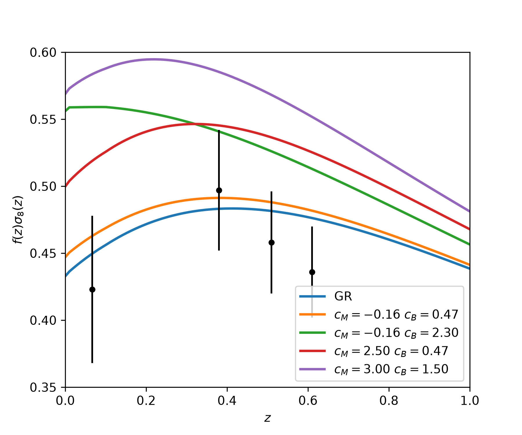
Figure 2: modifications of $f(z)\sigma_8(z)$ in Horndeski theories. Computed with a tutorial notebook.

Furthermore, Hordneski theories will impact the lensing and the ISW of the CMB through modification of $\Sigma$ as:

\[\Sigma(z) = \frac{1}{8\pi G M_*^2}\left(1 + \frac{\left(\alpha_M+\frac{\alpha_B}{2}\right)\left(2\alpha_M + 2\alpha_B\right)}{c_s^2\left(\alpha_K+\frac{3}{2}\alpha_B^{2}\right)}\right), \qquad \eta(z) = \frac{c_s^2\left(\alpha_K+\frac{3}{2}\alpha_B^{2}\right) + \alpha_B\left(\alpha_M+\frac{\alpha_B}{2}\right)}{c_s^2\left(\alpha_K+\frac{3}{2}\alpha_B^{2}\right) + 2\left(\alpha_M+\frac{\alpha_B}{2}\right)^{2}}\]

Hence, it is expected that the combination of growth of structure with galaxy surveys, combined with CMB and weak lensing surveys will maximally constrain the luminal Horndeski models.

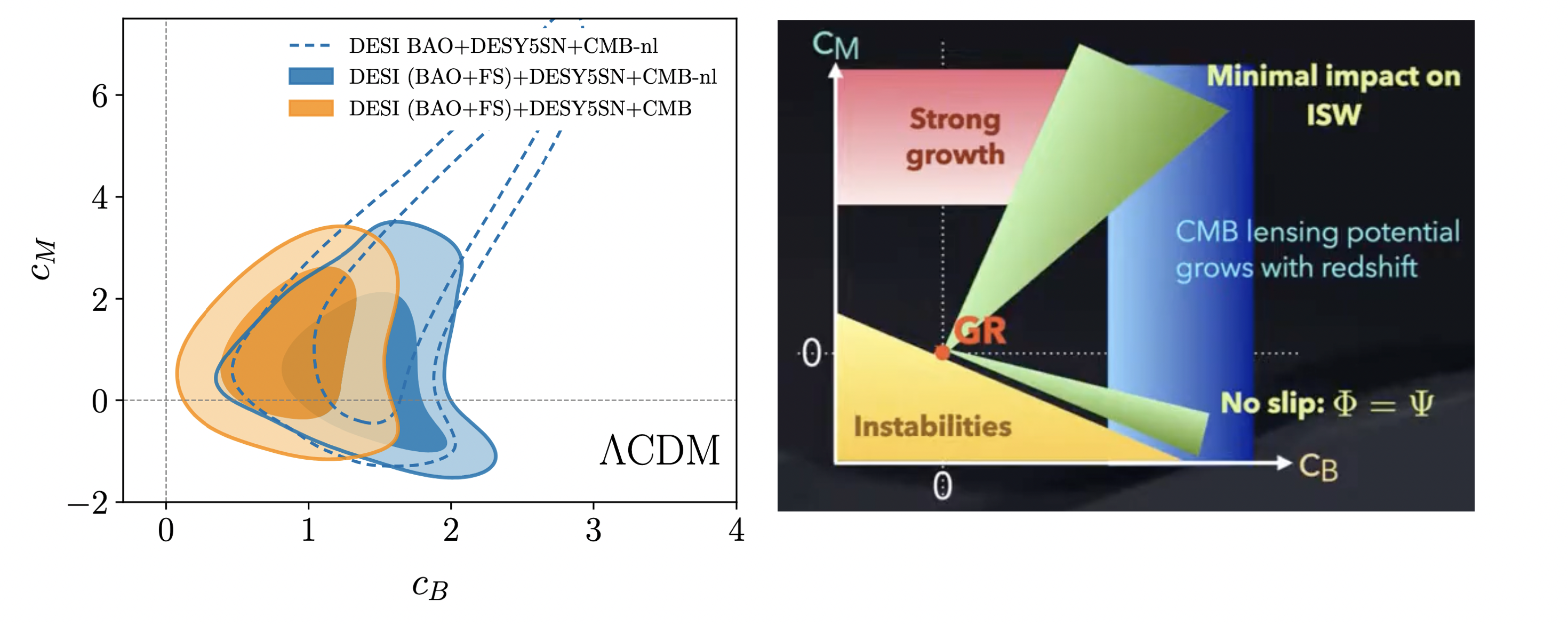
Figure 3: Left: constraints on the $\alpha_M$ $\alpha_B$ parametrisation from Ishak et al. (2024). Right: sketch to understand the figure, from Baker (2025).

A combination of data constraints on the $c_M$, $c_B$ space can be found on the left panel of Figure 3. As a reminder, these assumes the dark energy dependent parametrization of the coefficients $\alpha_M$ and $\alpha_B$ respectively. A sketch explaining the figure is available on the right panel. The lower left corner is forbidden by instabilities of the theories (yellow on the right sketch). Then, the ISW effect on the low $\ell$ plateau of the CMB $TT$ spectrum constrains strongly the data to prefer the diagonal lines (green on the right sketch). All the upper region of the panel is constrained by the measurement of growth of structures (red region on the sketch). The addition of DESI Full shape (FS) data containing the information on the galaxy clustering cuts the contour in regions that were unconstrained by CMB and narrow it to a significantly smaller region (from dashed blue to filled blue on the left plot). Finally the addition of CMB lensing (from blue to orange in the left plot), further constrain the parameter space (blue region on the right sketch).

One obtains $c_M = 1.05 \pm 0.96$ and $c_B = 0.092 \pm 0.33$ using DESI (FS + BAO) + DESY5SN + CMB (Ishak et al. (2024)) and the mild tension with GR disappears when one adds ISW galaxy-CMB cross correlations to reach $c_M = 0.12^{+0.28}_{-0.29}$ and $c_B = 0.54^{+0.9}_{-0.6}$ (Seraille et al. (2024)).

Local constraints

Now, you may wander about the PPN parameters and the local (solar system) constraints on Horndeski theories. Such a discussion will require the understanding of the complex screening mechanisms wich might allow such theories to devellop strong deviations from GR on cosmological scales while remaining hidden in solar system tests. We already mentioned that such effect would be hidden in terms as the $G_3$ function, but we will have to wait for the full dedicated lecture class to explore this in details.

Beyond Horndeski

In Figure 1, Horndeski models are in purple. While you might feel that we covered a lot of the modified gravity possibilities with Horndeski, we actually barely scratched the surface of the “extra-field” theories.
Second-order field equations is sufficient but not necessary for ghost-freedom; what is really needed is a degenerate kinetic matrix — that is, higher derivatives may appear provided they are not independent, so that no extra (ghostly) degree of freedom is actually propagated. This gives:

GLPV / “beyond Horndeski” (Gleyzes, Langlois, Piazza, Vernizzi 2015): adds two new possible terms to the Lagrangian $\mathcal{L}_4^{\rm bH}=F_4\,\epsilon^{\mu\nu\rho}{}_{\sigma}\epsilon^{\alpha\beta\gamma\sigma}\phi_\mu\phi_\alpha\phi_{\nu\beta}\phi_{\rho\gamma}$ and an $\mathcal{L}_5^{\rm bH}$.
DHOST / EST (Langlois & Noui 2016; Crisostomi, Koyama, Tasinato 2016): the full degenerate higher-order class, classified systematically by the rank of the degeneracy conditions.

The physical price of leaving Horndeski is that the Vainshtein screening becomes partially broken inside matter: the fifth force is suppressed outside a body but not within it, which produces observable signatures in stellar structure and in the profiles of galaxy clusters — and therefore new ways to test the models rather than merely new freedom.

Generalised Proca theories

If a scalar is allowed, why not a vector? The natural question is: what is the most general theory of a massive vector field $A_\mu$ with derivative self-interactions and second-order field equations? The answer is generalised Proca theory (Heisenberg 2014).

The logic parallels Horndeski exactly, with one extra subtlety. A massless vector has $2$ polarisations, protected by the $U(1)$ gauge symmetry $A_\mu\to A_\mu+\partial_\mu\lambda$. Giving it a mass breaks that symmetry and liberates a third, longitudinal mode. The danger is that generic self-interactions liberate a fourth — the temporal component $A_0$, which is a ghost, since it has no time derivative in the Maxwell kinetic term. Generalised Proca is the set of interactions arranged so that exactly 3 vector modes propagate (2 transverse + 1 longitudinal), giving $3+2=5$ degrees of freedom in total.

\[\mathcal{L}_{\rm GP} = \sum_{n=2}^{6}\mathcal{L}_n, \qquad X \equiv -\tfrac12 A_\mu A^\mu, \quad F\equiv -\tfrac14 F_{\mu\nu}F^{\mu\nu},\]

with five free functions $G_2(X,F,\ldots)$, $G_3(X)$, $G_4(X)$, $G_5(X)$, $G_6(X)$. Two structural facts are worth remembering:

The scalar limit is Horndeski. Taking $A_\mu\to\partial_\mu\pi$ (the longitudinal mode alone, the “decoupling limit”) reduces generalised Proca to the Galileons. The vector theory contains the scalar one.
Fewer free functions than Horndeski, because gauge structure constrains what can appear: the $G_i$ depend on $X$ only, not on $A_\mu$ separately.

Phenomenologically, generalised Proca admits self-accelerating de Sitter solutions with no potential and no cosmological constant — the acceleration comes from the vector’s derivative self-interactions — and supports black holes with vector hair, evading the usual no-hair theorems. As with Horndeski, GW170817 constrains the sector responsible for $c_T\neq c$ (here $\mathcal{L}_5$ and $\mathcal{L}_6$). Extensions exist: beyond-generalised Proca (Heisenberg, Kase & Tsujikawa 2016) and non-abelian generalised SU(2) Proca.

Tensor-Vector-Scalar gravity

All the theories above take dark matter for granted and modify gravity to explain dark energy. TeVeS (Bekenstein 2004) attacks the other problem: it is an attempt to do without dark matter altogether.

As discussed in the cosmology class, the motivation is MOND (Milgrom 1983): the observation that galaxy rotation curves flatten precisely when the Newtonian acceleration drops below a universal scale $a_0\simeq1.2\times10^{-10}\,\mathrm{m\,s^{-2}}$, where the dynamics is well described by $a=\sqrt{a_0\,g_N}$. This single rule reproduces the flat rotation curves and the baryonic Tully–Fisher relation with remarkable accuracy and no free parameter per galaxy — which is more than can be said for a dark-matter halo fit. But MOND as stated is a non-relativistic prescription: it has nothing to say about lensing, cosmology, or the CMB.

TeVeS is a relativistic completion. It carries three fields — the metric $g_{\mu\nu}$, a unit timelike vector $U_\mu$ (with $g^{\mu\nu}U_\mu U_\nu=-1$), and a scalar $\phi$ — and matter couples not to $g_{\mu\nu}$ but to a disformally related metric,

\[\tilde g_{\mu\nu} = e^{-2\phi}g_{\mu\nu} - 2\sinh(2\phi)\,U_\mu U_\nu .\]

Now why the vector is not optional? This is the most instructive feature of the theory, and it connects directly to Nordström’s theory: a purely conformal relation $\tilde g_{\mu\nu}=e^{-2\phi}g_{\mu\nu}$ cannot bend light at all, because null geodesics are conformally invariant. A scalar alone therefore produces extra gravitational attraction on matter but zero extra lensing — precisely the failure that killed Nordström’s theory in 1919. Since galaxy clusters lens far more strongly than their baryons can account for, any relativistic MOND must break conformal invariance. The vector $U_\mu$ is what supplies the disformal piece $U_\mu U_\nu$, singling out a preferred time direction and allowing light to feel the modification.

However, TeVeS in its original form is essentially dead:

it predicts $c_T\neq c$, and was excluded by GW170817 within days (Boran et al. 2018);
it struggles with the third acoustic peak of the CMB and with the offset between mass and baryons in the Bullet Cluster.

The story does not end there, however. AeST (Aether-Scalar-Tensor, Skordis & Złośnik 2021) is a modern successor which recovers MOND in galaxies, propagates gravitational waves at exactly $c$, and — unlike every previous relativistic MOND — reproduces the full CMB angular power spectrum and the matter power spectrum as well as $\Lambda$CDM. It does so at a price worth noting honestly: on cosmological scales its extra fields behave much like dust, so it does not so much abolish dark matter as replace it with something that behaves like dark matter where dark matter works and like MOND where MOND works. Whether that counts as an explanation or a re-description is a genuienly open question.