Why scalar fields?
In our previous class on whether GR is a field theory, we considered only scalar fields in a standard flat Minkowski space-time and saw that GR can be understood as a field theory for a massless, self-interacting, spin-2 field on a flat space-time: the graviton. We will now discuss the possibility that scalar fields exist, on top of the graviton, possibly interacting with it.
Scalar field models thud propose to add one or several new dynamical entities given by a frame independent value of a real or complex number at every point of space-time. They are very common in the cosmological literature and are so often invoked because:
- They are easy to implement consistently without breaking the general covariance of the theory. As such, they allow to build phenomenological “toy models” providing simple solutions to most of the cosmological puzzles as the $H_0$ tension, dark matter, inflation and so on. From the point of view of effective field theory (EFT), they can also reproduce the effective behavior of a more complicated underlying dynamics. They thus provides both simple and consistent modeling in order to seek for effects going beyond the SM, as varying dark energy, modification of gravity or possible variations of the fundamental constants of nature.
- Due to Lovelock theorem, we know adding new fields represent one of our only options to go beyond GR. Moreover, multiple higher order terms modifications of the action of gravity. can be shown to be equivalent to the addition of one or several scalar fields coupled to gravity. Furthermore, the addition of new compact dimensions to space-time gives rise to scalar degrees of freedom in the higher dimensional metric. Overall, multiple phenomenological routes beyond GR thus lead to scalar fields.
- Furthermore, scalar fields appear as theoretical necessities in multiple high energy physics models beyond the SM as Kaluza-Klein or string theory. They indeed appear in dimensional compactification (scalar degrees of freedom appearing in dimensional reduction are called the radions and moduli fields in Kaluza-Klein and string theory respectively) but also as fundamental fields like members of the string spectra (as the string dilaton). As such, fundamental routes from deeper principles tend also to lead to the existence of scalar fields.
- We know for a fact that they can be part of nature’s building blocks as proved by the discovery of the Higgs boson, which is itself a complex scalar field.
However, if the presence of such a field were ever detected on cosmological scales, a change of high energy physics paradigm would have to be considered, in order to understand where this new entity could fit in the realm of gauge theories over curved space-time, as well as how this new field can remain yet undetected in local/particle physics experiments.
A scalar field in curved space-time: Quintessence
Simply adding a scalar field, like the Higgs-Boson, within the curved space-time of general relativity is arguably not a theory of modified gravity, if the scalar field is not coupled anyhow interestingly to the geometry of space-time. The scalar field is better understood as a new contribution to the matter components, through its stress energy tensor. Such solutions are often invoked for alternative dark energy sources beyond $\Lambda$ (usually called “quintessence” models), as a mechanism for cosmic inflation or even for dark matter with axion models. This is a first theoretical model every cosmologist should master in every aspect in order to explore more advanced theories of real modified gravity beyond GR.
If one wants to add a new entity present in the cosmological space-time, the most rigorous way to do so is to introduce it at the Lagrangian level. The total Lagrangian is thus
\[\boxed{\mathcal{L} = \frac{1}{16\pi G}(R[g]-2\Lambda) + \mathcal{L}_\phi[\phi,g] + \mathcal{L}_m[\psi,g]}\]where a single metric $g$ appears everywhere, in accordance with both the EEP and the SEP. We considered that the field does not interact with matter, hence there is no interaction Lagrangian \(\mathcal{L}_{\rm int}(\phi,\psi,g)\). We already encountered the kinetic and potential Lagrangian of a scalar field in a previous lecture:
\[\boxed{\mathcal{L}_\phi= - \frac{1}{2}\partial_\mu \phi\partial^\mu \phi - V(\phi)}\]In curved space-time, recall that the action to extremize is given by the integral with the volume form:
\[\boxed{S = \int \sqrt{-|g|} \mathcal{L} \text{d}^4x}\]where $\vert g\vert$ is the determinant of the metric. This is the crucial difference with the flat space-time case. We will have to keep track of this additional factor of $\vert g\vert$ in all our derivations.
Stress-energy tensor
Now, we can wonder what would be the energy density and the pressure that such a field would exert on cosmological scales. These two ingredients are crucial, as we saw that they are appearing in the Friedman equations, driving the time evolution of the scale factor. As for every other component of the universe, the pressure and energy density are encoded in the stress energy tensor of the field.
In General relativity/curved space-time, we already saw that the stress-energy tensor of a matter field (here $\phi$) is defined as:
\[T^{\phi}_{\mu\nu} = -\frac{2}{\sqrt{-|g|}}\frac{\delta S_\phi}{\delta g^{\mu\nu}}\]Using this expression, we derive that:
\[\boxed{T^{\phi}_{\mu\nu}= \partial_\mu \phi \partial_\nu \phi - g_{\mu\nu}\left(\frac{1}{2}g^{\rho \sigma}\partial_\rho \phi \partial_\nu \phi + V(\phi)\right)}\]Proof
We need
\[\delta S_\phi=\int \delta\!\left(\sqrt{\vert-g\vert}\,\mathcal{L}_\phi\right)\mathrm{d}^4x =\int\Big[]\sqrt{\vert-g\vert}\,\delta\mathcal{L}_\phi+\mathcal{L}_\phi\,\delta\sqrt{-\vert g\vert }\Big]\mathrm{d}^4x .\]We re-use the expression in the first class for the metric variation (used in the derivation of Einstein equations):
\[\delta \sqrt{-\vert g \vert}=-\tfrac12\sqrt{\vert-g\vert}\,g_{\mu\nu}\,\delta g^{\mu\nu}.\]Only the kinetic term contains the metric ($V(\phi)$ does not), and it contains it linearly:
\[\delta\mathcal{L}_\phi=\delta\!\left(-\tfrac12 g^{\mu\nu}\partial_\mu\phi\,\partial_\nu\phi\right) =-\tfrac12\,\partial_\mu\phi\,\partial_\nu\phi\;\delta g^{\mu\nu}.\](The field $\phi$ is held fixed: we vary the metric only.)
Combining these two equations, we get
\[\frac{1}{\sqrt{\vert-g\vert}}\frac{\delta S_\phi}{\delta g^{\mu\nu}} =-\tfrac12\,\partial_\mu\phi\,\partial_\nu\phi-\tfrac12\,g_{\mu\nu}\,\mathcal{L}_\phi .\] \[T^\phi_{\mu\nu}=-\frac{2}{\sqrt{\vert-g\vert}}\frac{\delta S_\phi}{\delta g^{\mu\nu}} =\partial_\mu\phi\,\partial_\nu\phi+g_{\mu\nu}\mathcal{L}_\phi =\partial_\mu\phi\,\partial_\nu\phi-g_{\mu\nu}\Big(\tfrac12 g^{\rho\sigma}\partial_\rho\phi\,\partial_\sigma\phi+V(\phi)\Big).\;\square\]From this we find that, if the field is isotropic and in a FLRW metric the field can be treated as a perfect fluid with density and pressure:
\[\boxed{ \begin{align} \rho_\phi &= \frac{1}{2}\dot{\phi}^2 + V(\phi)\\ p_\phi &= \frac{1}{2}\dot{\phi}^2 - V(\phi) \end{align} }\]Proof
We work with the flat FLRW metric as usual: \(\mathrm{d}s^2=-\mathrm{d}t^2+a^2(t)\,\delta_{ij}\mathrm{d}x^i\mathrm{d}x^j, \qquad g_{\mu\nu}=\mathrm{diag}\big(-1,a^2,a^2,a^2\big),\) where $a(t)$ is the scale factor and $t$ the cosmic time.
Homogeneity and isotropy of the background forbid any spatial dependence of the field, so $\phi=\phi(t)$ and
\[\partial_0\phi=\dot\phi,\qquad \partial_i\phi=0 \quad\Longrightarrow\quad g^{\rho\sigma}\partial_\rho\phi\,\partial_\sigma\phi=g^{00}\dot\phi^2=-\dot\phi^{\,2}.\]The bracket in the stress tensor therefore reduces to
\[\tfrac12 g^{\rho\sigma}\partial_\rho\phi\,\partial_\sigma\phi+V=-\tfrac12\dot\phi^{\,2}+V.\]Setting $\mu=\nu=0$ in the stress tensor:
\[T^\phi_{00}=(\partial_0\phi)^2-g_{00}\Big(-\tfrac12\dot\phi^{\,2}+V\Big) =\dot\phi^{\,2}+\Big(-\tfrac12\dot\phi^{\,2}+V\Big) =\tfrac12\dot\phi^{\,2}+V(\phi).\]Setting $\mu=i,\nu=j$: the first term vanishes since $\partial_i\phi=0$, so
\[T^\phi_{ij}=-g_{ij}\Big(-\tfrac12\dot\phi^{\,2}+V\Big)=g_{ij}\Big(\tfrac12\dot\phi^{\,2}-V\Big),\]Now we compare these results with a perfect fluid of energy density $\rho$ and isotropic pressure $p$ has, by definition:
\[T_{\mu\nu}=(\rho+p)\,u_\mu u_\nu+p\,g_{\mu\nu} \quad\Longleftrightarrow\quad \rho=T_{\mu\nu}u^\mu u^\nu=T_{00},\qquad T_{ij}=p\,g_{ij}.\]with the comoving velocity associated to an observer defined as \(u^\mu=(1,0,0,0)\).
By identification we thus find:
\[\rho_\phi=\tfrac12\dot\phi^{\,2}+V(\phi).\] \[p_\phi=\tfrac12\dot\phi^{\,2}-V(\phi).\]Equations of motion: The Klein-Gordon equation
Applying Euler-Lagrange to the Lagrangian gives the Klein-Gordon equation describing the evolution of the field with the expansion
\[\boxed{\partial_\mu\partial^\mu \phi + \partial_\mu\ln\left(\sqrt{-\vert g \vert}\right)\partial^\mu \phi + \partial_\mu(g^{\mu\nu})\partial_\nu \phi = \frac{\partial V}{\partial \phi}}\]Remember that the d’Alembertian $\partial_\mu\partial^\mu \phi = - (\partial_t^2)/c^2 \phi+ \partial_x^2 \phi$ is characteristic of wave propagations. The whole left-hand side can be simply noted \(\Box \phi \equiv \nabla_\mu \nabla^\mu\phi\), as it is the curved generalization of the d’Alembertian with covariant derivatives (note that even if $\nabla^\mu\phi=\partial^\mu \phi$ for a scalar field, the second covariant derivative act on a vector and thus will make some Christoffel symbols appear). In the rest of this lecture we will always use $\Box$ to talk about the curved d’Alembertian, which reduces to the flat d’Alembertian in Minkowski space-time.
Proof
The Euler-Lagrange equation extremizing the action for fields of the matter sector in curved space-time is (first lecture):
\[\partial_\mu \left(\frac{\partial (\sqrt{-\vert g \vert}\mathcal{L})}{\partial (\partial_\mu \phi)}\right) = \frac{\partial (\sqrt{-\vert g \vert}\mathcal{L})}{\partial \phi}\]Where, for scalar fields only $\nabla_\mu = \partial_\mu$. Now, in our case, we have for the left-hand side:
\[\partial_\mu \left(\frac{\partial (\sqrt{-\vert g \vert}\mathcal{L})}{\partial (\partial_\mu \phi)}\right) = -\frac{1}{2}\partial_\mu \left(\sqrt{-\vert g \vert}\frac{\partial( \partial_\nu \phi \partial^\nu \phi)}{\partial (\partial_\mu \phi)}\right)\]where we renamed the dummy summation index $\nu$ to distinguish it from the derivative index $\mu$. Now, the product rules gives:
\[\frac{\partial(\partial_\nu \phi \partial^\nu \phi)}{\partial (\partial_\mu \phi)} = \frac{\partial (\partial_\nu \phi)}{\partial (\partial_\mu \phi)}\partial^\nu \phi + \partial_\nu \phi \frac{\partial(\partial^\nu \phi)}{\partial (\partial_\mu \phi)}\]We can then use the metric to rewrite $\partial^\nu \phi = g^{\nu \sigma}\partial_\sigma\phi$. We get:
\[\begin{align} &\frac{\partial(\partial_\nu \phi)}{\partial (\partial_\mu \phi)}\partial^\nu \phi + \partial_\nu \phi \frac{\partial(\partial^\nu \phi)}{\partial (\partial_\mu \phi)} \\ &=\frac{\partial(\partial_\nu \phi)}{\partial (\partial_\mu \phi)}\partial^\nu \phi + \partial_\nu \phi \frac{\partial(g^{\nu \sigma}\partial_\sigma\phi)}{\partial (\partial_\mu \phi)} \\ &= \delta_{\nu\mu} \partial^\nu \phi + \partial_\nu\phi g^{\nu \sigma} \delta_{\sigma\mu} \\ &= \delta_{\nu,\mu} \partial^\nu \phi + \partial_\nu\phi g^{\nu \sigma} \delta_{\sigma\mu} \\ &= \partial^\mu \phi + \partial^\mu\phi\\ &= 2 \partial^\mu \phi \end{align}\]Putting this back in our original expression for the left-hand side of the Euler-Lagrange equation, we get:
\[\begin{align} \partial_\mu \left(\frac{\partial (\sqrt{-\vert g \vert}\mathcal{L})}{\partial (\partial_\mu \phi)}\right) &= -\frac{1}{2}\partial_\mu \left(\sqrt{-\vert g \vert}\frac{\partial( \partial_\nu \phi \partial^\nu \phi)}{\partial (\partial_\mu \phi)}\right) \\ &= -\partial_\mu \left(\sqrt{-\vert g \vert} g^{\mu\nu} \partial_\nu \phi\right)\\ &= -\left(\partial_\mu(\sqrt{-\vert g \vert})\partial^\mu \phi + \sqrt{-\vert g \vert} \partial_\mu\partial^\mu \phi + \sqrt{-\vert g \vert}\partial_\mu(g^{\mu\nu})\partial_\nu \phi\right) \end{align}\]Now, the right-hand side is simply:
\[\frac{\partial (\sqrt{-\vert g \vert}\mathcal{L})}{\partial \phi} = -\sqrt{-\vert g \vert}\frac{\partial V}{\partial \phi}\]as $V$ is the only part of $\mathcal{L}$ that depends on $\phi$ itself. Equating both sides in the Euler-Lagrange equation, we get:
\[\begin{align} \partial_\mu(\sqrt{-\vert g \vert})\partial^\mu \phi + \sqrt{-\vert g \vert} \partial_\mu\partial^\mu \phi + \sqrt{-\vert g \vert}\partial_\mu(g^{\mu\nu})\partial_\nu \phi & = \sqrt{-\vert g \vert}\frac{\partial V}{\partial \phi}\\ \partial_\mu\partial^\mu \phi + \frac{1}{\sqrt{-\vert g \vert}}\partial_\mu(\sqrt{-\vert g \vert})\partial^\mu \phi+ \partial_\mu(g^{\mu\nu})\partial_\nu \phi &= \frac{\partial V}{\partial \phi} \\ \partial_\mu\partial^\mu \phi + \partial_\mu\ln\left(\sqrt{-\vert g \vert}\right)\partial^\mu \phi + \partial_\mu(g^{\mu\nu})\partial_\nu \phi &= \frac{\partial V}{\partial \phi} \end{align}\]In flat space-time, the metric is the Minkowski metric ($g=\eta$) and hence $\sqrt{-\vert g \vert}=1$ and $\partial_\mu(g^{\mu\nu})=0$, such the two term additional terms depending on the metric are zero. However, if we consider the FLRW metric and a field that is isotropic $\phi(t)$, we get:
\[\boxed{\ddot{\phi} + 3H \dot{\phi} = -\frac{\partial V}{\partial \phi}}\]where dots denote time derivatives and $H=\dot{a}/a = \text{d}\ln(a)/\text{d}t$.
Proof
We consider now a FLRW space-time in some co-moving coordinates, such that the field can be expressed locally as a function $\phi(t,x,y,z)$ and the metric as $g_{\mu\nu}=\text{diag}(-1,a^2,a^2,a^2)$ and $g^{\mu\nu}=\text{diag}(-1,1/a^2,1/a^2,1/a^2)$. If we now assume that the field is isotropic (or that its variations in space are so small that they can be neglected) it is represented by a function of time only, $\phi(t)$. Hence
\[\partial_\mu\partial^\mu\phi = g^{\mu\nu}\partial_\mu\phi\partial_\nu\phi = -(\partial_t)^2\phi + (\partial_x/a)^2\phi + (\partial_y/a)^2\phi + (\partial_z/a)^2\phi = -(\partial_t)^2\phi = -\ddot{\phi}.\]Furthermore, in the FLRW metric $\vert-g \vert=-a^6$ (recall that the determinant of a diagonal matrix is just the product of all of its entries). Hence, $\sqrt{-\vert g \vert} = \sqrt{-\vert g \vert}= a^3$ and $\ln(\sqrt{-\vert g \vert})=3\ln(a)$. Thus
\[\partial_\mu\ln(\sqrt{-\vert g \vert})\partial^\mu \phi=3 \partial_t\ln(a)g^{00}\dot{\phi}= -3H\dot{\phi}.\]Furthermore,
\[\partial_\mu(g^{\mu\nu})\partial_\nu \phi = \partial_t(-1)\partial_t\phi + \partial_x\left(\frac{1}{a^2(t)}\right)\partial_x\phi + \partial_y\left(\frac{1}{a^2(t)}\right)\partial_y\phi + \partial_z\left(\frac{1}{a^2(t)}\right)\partial_z\phi =0\]Putting everything together, we get:
\[\partial_\mu\partial^\mu \phi + \partial_\mu\ln\left(\sqrt{-\vert g \vert}\right)\partial^\mu \phi + \partial_\mu(g^{\mu\nu})\partial_\nu \phi = -\ddot{\phi} - 3H \dot{\phi}\]which in the Klein-Gordon equation gives
\[\begin{align} -\ddot{\phi} - 3H \dot{\phi}&= \frac{\partial V}{\partial \phi}\\ \ddot{\phi} + 3H \dot{\phi} &= -\frac{\partial V}{\partial \phi} \end{align}\]The same result can be reached from the continuity equation using the expression for $\rho_\phi$ and $P_\phi$ or using the two Friedmann equations.
Deriving the Klein-Gordon equation from the continuity equation
In a previous lecture, we saw that the energy density $\rho$ of a component evolved in the FLRW metric as:
\[\dot{\rho} + 3H(1+w)\rho = 0\]For the scalar field $\rho_\phi = \dot{\phi}^2/2 + V$ and thus
\[\begin{align} 1+w &= 1+\frac{p_\phi}{\rho_\phi}\\ &= 1 + \frac{\dot{\phi}^2/2 - V}{\dot{\phi}^2/2 + V}\\ &= \frac{\dot{\phi}^2/2 + V}{\dot{\phi}^2/2 + V} + \frac{\dot{\phi}/2 - V}{\dot{\phi}^2/2 + V}\\ &= \frac{\dot{\phi}^2}{\dot{\phi}^2/2 + V} \end{align}\]As such, the continuity equation for a field is:
\[\begin{align} &\dot{\rho} + 3H(1+w)\rho = 0\\ & \frac{\text{d}}{\text{d}t}\left(\dot{\phi}^2/2 + V\right) + 3H \frac{\dot{\phi}^2}{\dot{\phi}^2/2 + V} \left(\dot{\phi}^2/2 + V\right)=0\\ & 2\dot{\phi}\ddot{\phi}/2 + \dot{V} 3H \dot{\phi}^2 = 0\\ & \dot{\phi}\ddot{\phi} + \frac{\partial V}{\partial \phi}\dot{\phi} + 3H \dot{\phi}^2 =0\\ &\ddot{\phi} + 3H \dot{\phi} = -\frac{\partial V}{\partial \phi} \end{align}\]Deriving the Klein-Gordon equation from the Friedmann equations
The first Friedmann equation is
\[H^2 = \frac{8\pi G}{3}\rho\]in the case where a scalar field dominates the expansion, we get
\[H^2 = \frac{8\pi G}{3}(\dot{\phi}^2/2+V)\]Taking the time derivative of this equation, we obtain
\[2H\dot{H} = \frac{8\pi G}{3}(\dot{\phi}\ddot{\phi}+\frac{\partial V}{\partial \phi}\dot{\phi})\]Furthermore, the acceleration equation is
\[\dot{H} + H^2 = -\frac{4\pi G}{3}(\rho + 3p)\]which, for a scalar field alone is:
\[\begin{align} \dot{H} + H^2 &= -\frac{4\pi G}{3}(\dot{\phi}^2/2+V + 3\dot{\phi}^2/2 - 3V)\\ &= -\frac{4\pi G}{3}(2\dot{\phi}^2 -2V)\\ &= -\frac{8\pi G}{3}(\dot{\phi}^2 -V) \\ \end{align}\]and thus
\[\begin{align} \dot{H} &= -\frac{8\pi G}{3}(\dot{\phi}^2 -V) - H^2\\ &= -\frac{8\pi G}{3}(\dot{\phi}^2 -V) - \frac{8\pi G}{3}(\dot{\phi}^2/2+V)\\ & = -\frac{8\pi G}{3} \frac{3}{2} \dot{\phi}^2\\ & = -4\pi G \dot{\phi}^2 \end{align}\]Inserting this in the left hand-side of our previous derivation, we obtain
\[\begin{align} 2\dot{H}H &= \frac{8\pi G}{3}(\dot{\phi}\ddot{\phi}+\frac{\partial V}{\partial \phi}\dot{\phi})\\ - 8\pi G H\dot{\phi}^2 &= \frac{8\pi G}{3}(\dot{\phi}\ddot{\phi}+\frac{\partial V}{\partial \phi}\dot{\phi})\\ -3H\dot{\phi} &= \ddot{\phi} + \frac{\partial V}{\partial \phi}\dot{\phi} \end{align}\]Which is our Klein-Gordon equation!
On Mach’s principle and inertia
Mach’s principle(s)
Inertia is the property of a body to resist acceleration. In Newtonian language: apply the same force $\vec{F}$ to two different bodies and they acquire different accelerations, \(\vec{a} = \frac{\vec{F}}{m_i},\) the difference being carried entirely by the inertial mass $m_i$, which is the number quantifying inertia. As we already discussed, it is deeply puzzling that this $m_i$ should coincide with the gravitational mass $m_g$ — the gravitational charge of the body, appearing in $\vec{F}_{g} = m_g\,\vec{g}$. The two notions have nothing to do with one another a priori: one is a resistance to being pushed, the other a coupling strength to a field, exactly as electric charge $q$ in $\vec{F} = q\vec{E}$ is logically independent of $m_i$. Yet as we saw experiment finds them equal to one part in $10^{15}$ (Touboul et al. 2022). This is the weak equivalence principle (WEP). As we saw in our first lecture, promoting the WEP and supplementing it with local Lorentz invariance and local position invariance yields the Einstein equivalence principle (EEP), from which gravitation can be reinterpreted as a geometric phenomenon and GR constructed. But notice what has happened: GR does not explain the WEP, it postulates it1. And it says nothing about where inertia comes from in the first place. Both questions are simply built into the foundations.
The classic entry point into the question of the origin of inertia is Newton’s Scholium to the Definitions in the Principia (1687). Hang a bucket of water from a twisted rope and follow four successive states: Initially both bucket and water are at rest, and the surface is flat. Then the rope is released and the bucket begins to spin, but the water — viscosity not yet having acted — remains at rest: the surface is still flat, even though the water and the bucket are now in maximal relative rotation. After a while the water has been dragged into co-rotation with the bucket, so that their relative rotation has returned to zero — and it is precisely now that the surface becomes concave. Finally, stop the bucket abruptly. The water keeps rotating, relative rotation is once again maximal, and the surface remains concave. The curvature of the surface is therefore anti-correlated with the rotation of the water relative to its immediate material surroundings: it is absent when that relative rotation is maximal, and present when it vanishes. Whatever the water is rotating with respect to, it is not the bucket. Similar argument can follow by considering two globes joined by a cord, alone in an otherwise empty universe. If the pair spins about the midpoint of the cord, the tension in the cord reveals the rotation — even though, by construction, there is nothing to rotate relative to. (A point to be careful about. The tension comes from centripetal acceleration, not from relative motion as such. Two globes drifting apart along a straight line at constant velocity feel no steady tension: once the cord goes taut it simply decelerates them, and the motion is no longer inertial. It is genuinely essential that the motion be accelerated (here, circular). Newton’s argument is about acceleration, never about velocity.)
Newton thus concludes that the water and the globes rotate with respect to absolute space, a structure that exists independently of matter. Thus this discussion is deeply related to whether or not space(-time) exists by itself once every matter is gone (absolute), or if space-time is simply the relation between different objects and thus meaningless when everything has been removed (relative).
Ernst Mach’s rediscussed (much later) Newton’s points with famous counter-arguments (Die Mechanik in ihrer Entwicklung, 1883): Newton has shown only that the bucket is the wrong reference — a few kilograms of brass a few centimeters away. He silently held the rest of the universe fixed or empty. So: hold the bucket fixed and rotate all the matter of the universe around it — would the surface curve? If yes, the experiment proves nothing about absolute space; it proves that inertia is conferred by the rest of the matter in the universe. Nobody can perform that experiment, which is exactly Mach’s point: “absolute space” is an unfalsifiable placeholder for “the mean rest frame of cosmic matter”.
These ideas influenced Einstein considerably in his construction of GR — he coined the very name “Mach’s principle” (Einstein 1918) and declared its satisfaction “unconditionally necessary”. It is worth adding, though, that he later gave up on it: once de Sitter exhibited solutions whose metric is not determined by the matter content, Einstein progressively conceded that the metric field is a dynamical player in its own right, and by 1954 he was writing to Pirani that one should not speak of Mach’s principle at all (see Brown & Lehmkuhl 2013 for the history).
Mach’s principle however does not exist in a single unambiguous form. Mach never wrote an equation, and the literature contains a dozen mutually inequivalent statements. See for example, Bondi & Samuel (1997) who list eleven, Mach0 to Mach10, and show that two of them (Mach3 and Mach10) make opposite predictions for experimental effects as the sign of the Lense–Thirring effect (discussed below). We will use their labelling in what follows. There is a genuine empirical fact underlying all of this, and it deserves to be isolated from the philosophy:
- Mach0 (an observation, not a principle): locally, one can define a preferred inertial frame defined by local physics: non precessing gyroscopes or more accurately a zero Sagnac shift, which is a modern experiment allowing to test if one’s frame rotates. This frame coincides, to observational accuracy, with the frame in which the distant galaxies do not rotate.
This might seem trivial, but nothing in GR requires these two frames to agree. That they do is the whole motivation for what follows. For our discussion here, we shall use another version which is:
- Mach’s principle (Mach6-like): the inertia of a body is determined by its interaction with all the other bodies in the universe with which it is causally connected (i.e. within its observable universe).
So the question “is GR Machian?” is ill-posed until one specifies the version. We will not survey all this discussion here; for reviews see Bondi & Samuel (1997), the volume edited by Barbour & Pfister (1995), and Pfister & King (2015).
In GR, velocity is unambiguously relative: “$\vec{v}$” is meaningless until one says with respect to what. Formally, the coordinate 3-velocity of a worldline $x^\mu(\tau)$ is \(v^i = \frac{dx^i}{dt} = \frac{u^i}{u^0}, \qquad u^\mu \equiv \frac{dx^\mu}{d\tau},\) with $\tau$ the proper time and $u^\mu$ the 4-velocity. The statement $v^i = 0$ (equivalently $u^i = 0$) is coordinate-dependent: a change of chart, or simply a boost, makes it false. There is no such thing as absolute velocity. Acceleration is different. From the geodesic equation, we can define its deviation to be the 4-acceleration
\[a^\mu = u^\nu \nabla_\nu u^\mu\]is a tensor. Whether it vanishes is therefore a coordinate-independent, observer-independent fact, and — crucially — it is measured locally, by an accelerometer in a sealed box, with no reference to anything external. The same holds for rotation: a gyroscope, or a Sagnac interferometer detects rotation without ever looking at the sky. So acceleration looks absolute. But the statement needs one refinement, and it is the crux of the whole debate: $a^\mu$ measures acceleration relative to the local inertial frames, and those frames are determined by the metric $g_{\mu\nu}$ — which is itself sourced, at least in part, by matter. GR is therefore partly Machian: a rotating body genuinely drags local inertial frames along with it (the Lense–Thirring effect, Lense & Thirring 1918, measured to ~19% by Gravity Probe B), and inside a rotating shell approaching its own Schwarzschild radius the dragging becomes total (Brill & Cohen 1966) — exactly what Mach asked for. The problem is that matter does not determine the metric completely. Einstein’s equations admit solutions with $T_{\mu\nu} = 0$ everywhere: Minkowski space, Schwarzschild, Kerr, gravitational waves in vacuum. In Minkowski space an isolated test body has full inertia and there is nothing whatsoever for it to be inertial with respect to.
The precise statement is worth making carefully, because “vacuum solutions exist” is a slightly blunt way to put it. $G_{\mu\nu} = 8\pi G\,T_{\mu\nu}/c^4$ is a system of differential equations: solving it requires initial and boundary data in addition to $T_{\mu\nu}$, and those data are not fixed by the matter content. This is exactly the lesson Einstein drew from de Sitter’s solution. In an asymptotically flat spacetime the boundary condition (flatness at infinity) is itself an absolute element of the theory in the technical sense — a structure that is not varied and not determined by anything. So GR fails what Bondi would call Mach9 (“no absolute elements”) in that setting, and it fails their Mach2 (“an isolated body in empty space has no inertia”) outright. An even sharper example, since it does not rely on emptiness: the Gödel universe is a solution with matter everywhere, in which the matter rotates relative to the local inertial frames. Mach0 — the observed alignment of the two frames — is thus not a theorem of GR, but a contingent feature of our universe.
The conclusion is uncomfortable: in GR, Newton’s absolute space and time appear to have been replaced by an absolute curved spacetime, still endowed with an inertial structure that matter does not fully dictate. Whether this is a defect to be repaired or simply the correct description of nature remains actively debated; see Barbour & Pfister (1995), Pfister & King (2015), and, for the historical and conceptual side, Brown & Lehmkuhl (2013) and the Stanford Encyclopedia entry on absolute and relational space and motion.
Mach’s principle(s) and a varying $G$
Now, and this connects to the rest of our lecture: a varying $G$ was proposed and motivated as a way to implement Mach’s principle. There are several ways to motivate this, unfortunately mostly flirting with numerology. Imagine that inertia is nothing else than a form of gravitational attraction with the rest of the universe, felt by each body. The rest energy of a test body of inertial mass $m_i$ is $m_i c^2$ and the gravitational potential of the universe at the position of the test body is \(\Phi_U \;=\; -\,G\sum_k \frac{m_k}{r_k},\) with the sum running over every body $k$, of mass $m_k$ and distance $r_k$, with which the test body can interact gravitationally. The corresponding interaction energy of our test body is $m_g \Phi_U$ — it carries a factor of the body’s gravitational mass. Now suppose that inertial energy is nothing more than the gravitational energy of the interaction of the body with the rest of the universe, we get \(m_i c^2 \;=\; m_g\,\vert\Phi_U\vert\), or in other words \(m_i \;=\; \chi\, m_g\) with
\[\chi \;\equiv\; \frac{|\Phi_U|}{c^2} \;=\; \frac{G}{c^2}\sum_k\frac{m_k}{r_k}.\]We have derived that $m_i$ is proportional to $m_g$, meaning that the ratio $m_i/m_g$ is the same universal number $\chi$ for every body, whatever it is made of. Now, we have good observational reasons (UFF) to believe that \(m_i =m_g\) and the current theory is encouraging us to think so: since inertia becomes just a form of gravitational attraction the two concepts might very well be the same: they are gravitational charges. Under these conditions, we obtain:
\[\boxed{\ \chi \;=\; \frac{G}{c^2}\sum_k\frac{m_k}{r_k}\;\simeq\;1\ }\]However we might as well never use the equivalence principle as a postulate and consider the equation above instead as cosmological condition that should be satisfied in our Universe.
Now, it is easy to show that a static classical Newtonian potential cannot produce the required effect and be the source of inertia. What we need is a force proportional to the relative acceleration between the body and the distant matter — and a $1/r$ potential, which depends only on positions, cannot generate one. Sciama (1953) proposed a toy model in which gravity is mediated by a vector field, like electromagnetism. Just as Maxwell’s theory has a vector potential $\vec A$ whose time derivative contributes to $\vec E$ (induction), Sciama’s theory contains an inertial induction term proportional to the acceleration of the distant bodies — exactly what is needed. This is of course not a correct theory of gravity: we saw before that gravity cannot be propagated by a spin-1 field. But it has the merit of showing that if some form of induction is added to gravity, the desired Machian effect can be produced. In order for the WEP to be valid, Sciama’s theory also requires exactly that $\chi \sim 1$.
If $\chi \simeq 1$, we can rewrite the condition as
\[\boxed{\frac{1}{G} \;\simeq\; \frac{1}{c^2}\sum_k \frac{m_k}{r_k}}\]so that $G$ is no longer an unexplained dimensional constant of the theory, but a dynamical quantity, varying from point to point in spacetime, quantifying all the bodies in the observable universe with which that point can interact to make its inertia. Hence: $G$ is small because the universe is large.
Coarse-graining the sum over a homogeneous medium of density $\rho$, the contribution of the shell $[r, r+dr]$ is \(d\!\left(\sum_k \frac{m_k}{r_k}\right) = \frac{4\pi\rho\,r^2dr}{r} = 4\pi\rho\,r\,dr,\) which grows linearly with $r$: mass accumulates as $r^3$ while the $1/r$ suppression removes only one power. The sum is therefore dominated by the most distant matter. Computing this integral gives $7\times10^{-10}$ at Earth surface, $1\times10^{-8}$ at 1 AU from the sun, $\sim 6\times10^{-7}$ at 8 kpc from the Milky way and $\sim 1$ for the observable Universe. This is the quantitative content of Mach’s intuition: whatever fixes your inertia, it is not your neighbours. Local physics is essentially blind to local matter and sensitive only to the cosmological total — which is also why $\chi$ can be treated as a single universal number, the same for all bodies, as assumed above.
What is fascinating is that the relation holds on cosmological scales as a matter of observational fact. Take the Hubble radius $R_H \equiv c/H_0$, with $H_0$ the present expansion rate, to represent the size of the observable Universe. (Indeed, this corresponds to the total distance travelled by light \(R_H = c \Delta t\) since the birth of our Universe. Assuming a constant expansion rate $\dot{a}/a=H_0$ through all its history from $a=0$ to $a=1$, we get \(H_0= \frac{1}{a}\Delta a / \Delta t = 1/\Delta t\)). Estimating the total mass as $M_{\rm tot} = \frac{4}{3}\pi\rho R_H^3$, we get:
\[\chi \simeq \frac{GM_{\rm tot}}{R_H c^2} = \frac{4\pi G\rho R_H^2}{3c^2} = \frac{4\pi G \rho}{3H_0^2}.\]Now compare with the critical density $\rho_c \equiv \dfrac{3H_0^2}{8\pi G}$ and the density parameter $\Omega_{\rm tot} \equiv \rho/\rho_c$:
\[\boxed{\ \chi \simeq \frac{\Omega_{\rm tot}}{2}\ }\]So $\chi$ is half the total density parameter. Observationally $\Omega_{\rm tot} = 1.000 \pm 0.002$ (Planck 2018), hence $\chi \sim 1$. The Friedmann equation gives \(\Omega_{\rm tot} - 1 = \frac{Kc^2}{a^2H^2},\) i.e. $\Omega_{\rm tot} = 1$ is equivalent to spatial flatness ($K=0$). That the universe is observed to be flat to $\Omega_K = 0.0007\pm0.0019$ is itself a puzzle (the flatness problem), which is one of the motivations for inflation. So the Machian coincidence $\chi\sim1$ is not explained here — it is traded for the flatness problem.
Note that $\chi \sim 1$ applied to the whole universe can be rewritten as
\[M_{\rm tot} c^2 \;\sim\; \frac{GM_{\rm tot}^2}{R},\]i.e. the rest energy of the universe is comparable to the magnitude of its own gravitational binding energy. Since gravitational potential energy is negative, this is the statement that the total energy of the universe may be close to zero — the “free lunch”, proposed by Tryon (1973) and popularised by Guth. Hence, particles could be created indefinitely “for free”, because their additional inertial energy would be exactly compensated by their contribution to the gravitational binding energy. In the Bondi–Samuel taxonomy this is Mach5: the total energy, linear and angular momentum of the universe vanish. So the Machian condition and the zero-total-energy condition are the same order-of-magnitude statement seen from two directions. This discussion on large numbers inspired many authors, and notably led Dirac (1937) to propose along a different path that $G$ evolves through cosmic history, as we saw in another lecture.
So: all of this is very much numerology, and one needs a concrete and viable theory of gravitation in which the ideas can be made precise. The attempt to do so is the scalar–tensor field theory of Brans & Dicke (1961), to which we now turn — where $1/G$ becomes a genuine field $\phi$.
(Jordan)-Brans-Dicke theory
The theory
So far $\chi = 1$ is a relation between numbers, not a theory. It becomes dynamics in Brans-Dicke theory (Brans & Dicke 1961). This theory is the classical example of a deeply motivated theory going beyond GR that was unfortunately disproved by experiment. It inspired countless generalizations still studied today. Understanding all the fine details of this theory is thus extremely important, as it illustrates most of the concepts that will appear over and over again in other modern theories of gravity with extra fields. For a review on the history of this theory, see Brans (2005). The proposal is to replace $1/G$, the relevant quantity for Mach’s principle, by a dynamical quantity related to some new field. Since $G$ is a number, the simplest form is to say should that $1/G$ itself is a scalar field. Simply replacing $1/G$ by $\phi$ and adding a kinetic term for $\phi$ one obtains immediately the Lagrangian density:
\[\mathcal{L} = \frac{1}{16\pi}\phi R - \frac{1}{2}g^{\mu\nu}\partial_\mu\phi\,\partial_\nu\phi + \mathcal{L}_{m}[\psi,g],\]Note that we set \(\Lambda=0\) here for now, as in the original theory (long before the accelerated expansion was detected). We will come back to the question of how to include dark energy in such models in the Brans-Dicke cosmology section below. Now our Lagrangian can not be right, as the action must have the dimension of an energy times a time. Setting $c=1$, \([t]=[x]=L\) and energy has dimension of mas $M$. Hence \([S]=M.L\) and \([\text{d}x^4]=L^4\) so \([\mathcal{L}]=M/L^3\). $G$ has dimension \(M^{-1}.L^{3}.T^{-2}= L/M\) and thus \([\phi]=[1/G]=M/L\). The kinetic term thus have the wrong dimension of \(M^2/L^4\). The solution would be to multiply the kinetic by an unknown constant say $\kappa$ of dimension \(L/M\), in order to fix the dimensions. However, this goes against one of the ambition of our theory: to get read of unknown an unexplained dimensional values such as $G$. Brans and Dicke thus proposed the minimal fix:
\[\boxed{\mathcal{L} = \frac{1}{16\pi}\left(\phi R - \frac{\omega}{\phi}g^{\mu\nu}\partial_\mu\phi\,\partial_\nu\phi\right) + \mathcal{L}_{m}[\psi,g],}\]where $\omega$ is a dimensionless coupling known as the fudge factor and GR recovered as $\omega\to\infty$. The $1/16\pi$ factor multiplying the field’s kinetic Lagrangian is here largely for convention, but it will make future equations more convenient than a standard $1/2$ and it really ties the interpretation that we make of $\phi$ as a contribution to the gravity sector instead of an independent scalar field. Indeed, this is our first proper modified gravity theory! It might also be the simplest we could have thought about by simply promoting $G$ to a field and asking for a consistent action. We see that:
- Because of its coupling to $R$, the presence of the field will modify the laws of gravitation and thus the dynamics of gravity (D1). It goes around Lovelock theorem by adding a field to gravity beyond the metric, thus violating our GR axiom (S2) stating that $g$ is the only dynamical variable.
- As a varying $G$ theory, it should be equivalent to a theory in which matter responds to another metric than gravity (see our discussion in the dedicated class): it violates unavoidably the strong equivalence principle (SEP).
From the action, we can now compute the equations of motions and obtain, when varying with respect to the metric:
\[\boxed{\;G_{\mu\nu} = \frac{8\pi}{\phi}T_{\mu\nu} \;+\; \frac{\omega}{\phi^2}\left(\nabla_\mu\phi\nabla_\nu\phi - \tfrac12 g_{\mu\nu}\nabla^\alpha\phi\nabla_\alpha\phi\right) \;+\; \frac{1}{\phi}\Big(\nabla_\mu\nabla_\nu\phi - g_{\mu\nu}\Box\phi\Big)\;}\]This is clearly a modified Einstein equation (D1). The first term is simply Einstein equation with a varying $G$. But that’s not all! The two next terms can be understood as contribution of the field to the space-time geometry, both from its own energy and from its self interaction.
Proof
Before proceeding, we will need the following useful formulas:
-
Relation 1 (determinant variation): \(\delta\sqrt{-\vert g\vert} = -\tfrac12\sqrt{-\vert g\vert}\;g_{\mu\nu}\,\delta g^{\mu\nu}.\) which was proven in our first lecture.
-
Relation 2. : \(\phi \frac{\delta R}{\delta g^{\mu\nu}} =\phi R_{\mu\nu} + g_{\mu\nu}\Box \phi - \nabla_\mu\nabla_\nu\phi\) which is a generalization of the Palatini formula from the first lecture, in the presence of a field $\phi$.
Proof of relation 2
We start from the Palatini formula:
\[\delta R_{\mu\nu} = \nabla_\rho\,\delta\Gamma^\rho_{\mu\nu} - \nabla_\nu\,\delta\Gamma^\rho_{\rho\mu}.\]Contracting with $g^{\mu\nu}$ and expressing $\delta\Gamma$ in terms of $\delta g^{\mu\nu}$: \(g^{\mu\nu}\,\delta R_{\mu\nu} = g_{\mu\nu}\,\Box\,\delta g^{\mu\nu} - \nabla_\mu\nabla_\nu\,\delta g^{\mu\nu}.\) This whole term was vanishing in standard GR, as a boundary term. We will see that this will not be the case anymore in Brans Dicke theory, because of the presence of $\phi$.
Starting from $\Gamma^\rho_{\mu\nu} = \tfrac12 g^{\rho\lambda}(\partial_\mu g_{\lambda\nu} + \partial_\nu g_{\lambda\mu} - \partial_\lambda g_{\mu\nu})$,
We discussed already that while $\Gamma^\rho_{\mu\nu}$ is not a tensor, $\delta\Gamma^\rho_{\mu\nu}$ is. Hence its expression in a system of coordinate is true everywhere. Take Riemann normal coordinates at $p$: there $g_{\mu\nu}(p)=\eta_{\mu\nu}$, $\partial_\alpha g_{\mu\nu}(p)=0$ and \(\Gamma^\rho_{\mu\nu}(p)=0\). Varying the definition,
\[\delta\Gamma^\rho_{\mu\nu} = \tfrac12\,\delta g^{\rho\lambda}\underbrace{\left(\partial_\mu g_{\lambda\nu}+\partial_\nu g_{\lambda\mu}-\partial_\lambda g_{\mu\nu}\right)}_{=\;0\ \text{at}\ p} \;+\; \tfrac12 g^{\rho\lambda}\left(\partial_\mu\,\delta g_{\lambda\nu}+\partial_\nu\,\delta g_{\lambda\mu}-\partial_\lambda\,\delta g_{\mu\nu}\right).\]The first group vanishes at $p$, and since $\Gamma(p)=0$ we may replace $\partial\to\nabla$ in the second. This establishes (1) at $p$; tensoriality extends it everywhere. So:
\[\delta\Gamma^\rho_{\mu\nu} = \tfrac12\,g^{\rho\lambda}\left(\nabla_\mu\,\delta g_{\lambda\nu} + \nabla_\nu\,\delta g_{\lambda\mu} - \nabla_\lambda\,\delta g_{\mu\nu}\right)\;\]Contract now Palatini with $g^{\mu\nu}$. Because the connection is metric-compatible ($\nabla_\alpha g^{\mu\nu}=0$), the inverse metric slides freely through the covariant derivatives:
\[g^{\mu\nu}\delta R_{\mu\nu} = \nabla_\rho\!\left(g^{\mu\nu}\delta\Gamma^\rho_{\mu\nu}\right) - \nabla_\nu\!\left(g^{\mu\nu}\delta\Gamma^\rho_{\rho\mu}\right).\]Relabelling the dummy index on the second outer derivative, both terms become the divergence of a single vector:
\[\boxed{\;g^{\mu\nu}\delta R_{\mu\nu} = \nabla_\rho\,v^\rho\;},\qquad v^\rho \equiv g^{\mu\nu}\,\delta\Gamma^\rho_{\mu\nu} \;-\; g^{\rho\mu}\,\delta\Gamma^\nu_{\nu\mu}. \tag{3}\]This is already the structurally important fact: $g^{\mu\nu}\delta R_{\mu\nu}$ is a pure divergence. In GR it therefore integrates to a boundary term and is discarded — which is why the Einstein equations contain no derivatives of the metric beyond second order. All that remains is to write $v^\rho$ explicitly.
First, the trace part $\delta\Gamma^\nu_{\nu\mu}$. Set $\rho=\nu$ in our expression and sum:
\[\delta\Gamma^\nu_{\nu\mu} = \tfrac12 g^{\nu\lambda}\Big(\underbrace{\nabla_\nu\,\delta g_{\lambda\mu}}_{\text{(i)}} + \nabla_\mu\,\delta g_{\lambda\nu} - \underbrace{\nabla_\lambda\,\delta g_{\nu\mu}}_{\text{(iii)}}\Big).\]Terms (i) and (iii) cancel: $g^{\nu\lambda}$ is symmetric, so relabelling $\lambda\leftrightarrow\nu$ in (iii) turns it into (i). Only the middle term survives, and by metric compatibility it is a total derivative:
\[\boxed{\;\delta\Gamma^\nu_{\nu\mu} = \tfrac12\,g^{\nu\lambda}\nabla_\mu\,\delta g_{\lambda\nu} = \tfrac12\,\nabla_\mu\big(g^{\nu\lambda}\delta g_{\lambda\nu}\big) = \tfrac12\,\nabla_\mu\,(\delta g)\;}\tag{4}\]with $\delta g \equiv g^{\mu\nu}\delta g_{\mu\nu}$ as in (0b). Hence
\[g^{\rho\mu}\,\delta\Gamma^\nu_{\nu\mu} = \tfrac12\,\nabla^\rho(\delta g).\]Now, contract Palatini with $g^{\mu\nu}$:
\[g^{\mu\nu}\delta\Gamma^\rho_{\mu\nu} = \tfrac12 g^{\rho\lambda}\Big(\underbrace{g^{\mu\nu}\nabla_\mu\delta g_{\lambda\nu} + g^{\mu\nu}\nabla_\nu\delta g_{\lambda\mu}}_{\text{identical, by }\mu\leftrightarrow\nu} - g^{\mu\nu}\nabla_\lambda\delta g_{\mu\nu}\Big)\] \[= g^{\rho\lambda}g^{\mu\nu}\nabla_\mu\,\delta g_{\lambda\nu} \;-\; \tfrac12\,g^{\rho\lambda}\nabla_\lambda(\delta g) \;=\; g^{\rho\lambda}g^{\mu\nu}\nabla_\mu\,\delta g_{\lambda\nu} \;-\; \tfrac12\,\nabla^\rho(\delta g).\]We now assemble
\[v^\rho = g^{\rho\lambda}g^{\mu\nu}\nabla_\mu\,\delta g_{\lambda\nu} - \tfrac12\nabla^\rho(\delta g) - \tfrac12\nabla^\rho(\delta g) = \nabla_\mu\!\left(g^{\rho\lambda}g^{\mu\nu}\delta g_{\lambda\nu}\right) - \nabla^\rho(\delta g),\]where the metrics were pulled inside $\nabla_\mu$ using metric compatibility. Now convert to variations of the inverse metric with the identities — this is where the two minus signs enter:
- from the definition of the inverse metric: $\;g^{\rho\lambda}g^{\mu\nu}\delta g_{\lambda\nu} = -\,\delta g^{\rho\mu}$;
- by formula 1: $\;\delta \vert g\vert = -\,g_{\mu\nu}\delta g^{\mu\nu}$.
We now take the divergence Apply $\nabla_\rho$ to (5) — again $g_{\mu\nu}$ passes through freely:
\[\nabla_\rho v^\rho = -\,\nabla_\rho\nabla_\mu\,\delta g^{\rho\mu} \;+\; g_{\mu\nu}\,\nabla_\rho\nabla^\rho\,\delta g^{\mu\nu}.\]Rename the dummies in the first term ($\rho\to\mu,\ \mu\to\nu$) and recognize $\nabla_\rho\nabla^\rho=\Box$ in the second.
\[\boxed{\;g^{\mu\nu}\,\delta R_{\mu\nu} \;=\; g_{\mu\nu}\,\Box\,\delta g^{\mu\nu} \;-\; \nabla_\mu\nabla_\nu\,\delta g^{\mu\nu}\;}\]$\int\sqrt{-\vert g\vert}\,\phi\,g_{\mu\nu}\Box\,\delta g^{\mu\nu} = \int\sqrt{-\vert g\vert}\,(\Box\phi)\,g_{\mu\nu}\delta g^{\mu\nu}$ (self-adjointness of $\Box$), and $-\int\sqrt{-\vert g\vert}\,\phi\,\nabla_\mu\nabla_\nu\,\delta g^{\mu\nu} = -\int\sqrt{-\vert g\vert}\,(\nabla_\mu\nabla_\nu\phi)\,\delta g^{\mu\nu}$.
Multiplying by $\phi$ and integrating by parts twice (discarding boundary terms):
\[\int d^4x\sqrt{-\vert g\vert}\;\phi\,g^{\mu\nu}\delta R_{\mu\nu} = \int d^4x\sqrt{-\vert g\vert}\;\Big[g_{\mu\nu}\Box\phi - \nabla_\mu\nabla_\nu\phi\Big]\,\delta g^{\mu\nu}.\]Now, write $S = S_{grav} + S_{m}$ and vary term by term:
\[\delta S = \int\left(\frac{\delta \sqrt{-\vert g \vert}\mathcal{L}_{grav}}{\delta g^{\mu\nu}} \delta g^{\mu\nu} + \frac{\delta\sqrt{-\vert g \vert}\mathcal{L}_{m}}{\delta g^{\mu\nu}} \delta g^{\mu\nu}\right) \text{d}^4x = 0\]For it to vanish, this integral should be zero for all $\delta g^{\mu\nu}$, we get:
\[\frac{\delta \sqrt{-\vert g \vert}\mathcal{L}_{grav}}{\delta g^{\mu\nu}} + \frac{\delta\sqrt{-\vert g \vert}\mathcal{L}_{m}}{\delta g^{\mu\nu}}=0\]First, we focus on the gravitational part. Using the two relations above, we obtain:
\[\begin{align} \frac{\delta \sqrt{-\vert g \vert}\mathcal{L}_{grav}}{\delta g^{\mu\nu}} &= \frac{1}{16\pi}\frac{\delta}{\delta g^{\mu\nu}}\left(\sqrt{-\vert g \vert}\left(\phi R - \frac{\omega}{\phi}g^{\mu\nu}\partial_\mu \phi\partial_\nu \phi\right)\right)\\ &= \frac{1}{16\pi}\left(\frac{\delta{\sqrt{-\vert g \vert}}}{\delta g^{\mu\nu}} \left(\phi R - \frac{\omega}{\phi}g^{\mu\nu}\partial_\mu \phi\partial_\nu \phi\right) + \sqrt{-\vert g \vert}\left(\phi \frac{\delta R }{\delta g^{\mu\nu}}- \frac{\delta(\frac{\omega}{\phi}g^{\mu\nu}\partial_\mu \phi\partial_\nu \phi)}{\delta g^{\mu\nu}} \right)\right)\\ &= \frac{1}{16 \pi}\left( -\tfrac12\sqrt{-\vert g\vert}\;g_{\mu\nu}\left(\phi R - \frac{\omega}{\phi}g^{\mu\nu}\partial_\mu \phi\partial_\nu \phi\right) + \sqrt{-\vert g\vert}\left(\phi R_{\mu\nu} + g_{\mu\nu}\Box \phi - \nabla_\mu\nabla_\nu\phi- \frac{\omega}{\phi}\partial_\mu \phi\partial_\nu \phi\right) \right) \end{align}\]For the matter action, by definition of $T_{\mu\nu}$:
\[\;\frac{\delta \sqrt{-\vert g \vert}\mathcal{L}_{m}}{\delta g^{\mu\nu}} = -\tfrac12\sqrt{-\vert g\vert}\,T_{\mu\nu}\]Putting it all together and setting to zero:
\[\phi\Big(R_{\mu\nu}-\tfrac12 g_{\mu\nu}R\Big) - \frac{\omega}{\phi}\Big(\nabla_\mu\phi\nabla_\nu\phi - \tfrac12 g_{\mu\nu}(\nabla\phi)^2\Big) + g_{\mu\nu}\Box\phi - \nabla_\mu\nabla_\nu\phi = 8\pi T_{\mu\nu},\]where $(\nabla\phi)^2 \equiv \nabla^\alpha\phi\nabla_\alpha\phi$. Dividing by $\phi$, we obtain the desired equation:
\[\;G_{\mu\nu} = \frac{8\pi}{\phi}T_{\mu\nu} \;+\; \frac{\omega}{\phi^2}\left(\nabla_\mu\phi\nabla_\nu\phi - \tfrac12 g_{\mu\nu}\nabla^\alpha\phi\nabla_\alpha\phi\right) \;+\; \frac{1}{\phi}\Big(\nabla_\mu\nabla_\nu\phi - g_{\mu\nu}\Box\phi\Big)\;\]When varying the action with respect to the field, we obtain:
\[\boxed{\;\Box\phi = \frac{8\pi}{3+2\omega}\,\mathcal{T}\;}\]This reminds us of the scalar gravitation (Nordstrom) theory we already explored in a previous lecture. Hence, we see that matter sources the field through its stress energy tensor \(\mathcal{T}\) (there is no solution for which \(\mathcal{T}\neq 0\) and \(\phi=0\)). As in the action, taking the limit $\omega \to \infty$ gives $\Box\phi \to 0$: the scalar decouples from matter and the Einstein equation reduces to Einstein’s equations with $G = 1/\phi_0$. GR is recovered, and it is recovered because the scalar stops interacting with matter. As for Nordstrom theory: for radiation , $\mathcal{T} = 0$, so $\phi$ is not sourced at all. The Brans–Dicke scalar is blind to the radiation era. The value $\omega = -3/2$ is singular and the theory is pathological there.
Proof
Now vary the action with respect to $\phi$ at fixed $g_{\mu\nu}$. Since $\phi$ is absent from $S_{m}$, only $S_{grav}$ contributes. Using the classical rules we saw over and over again for action extremelisation (see here again):
\[\begin{align} \delta S &= \int \left(\frac{\delta \sqrt{-\vert g \vert}\mathcal{L}_{grav}}{\delta \phi}\delta \phi + \frac{\delta \sqrt{-\vert g \vert} \mathcal{L}_{grav}}{\delta (\partial_\mu\phi)}\delta(\partial_\mu\phi) \right)\text{d}^4 x = 0\\ &\int \sqrt{-\vert g \vert}\left(\frac{\delta \mathcal{L}_{grav}}{\delta \phi}\delta \phi + \frac{\delta \mathcal{L}_{grav}}{\delta (\partial_\mu\phi)}\delta(\partial_\mu\phi) \right)\text{d}^4 x = 0\\ & \int \sqrt{-\vert g \vert}\delta \phi\left(\frac{\delta \mathcal{L}_{grav}}{\delta \phi} - \frac{1}{\sqrt{-\vert g \vert}}\partial_\mu\left(\frac{\delta \sqrt{-\vert g \vert}\mathcal{L}_{grav}}{\delta (\partial_\mu \phi)}\right) \right) \text{d}^4 x =0\\ \end{align}\]Remember to avoid the classic mistake: $\sqrt{-\vert g\vert}$ is a function of $x$ so it cannot be pulled out of the integral and simplified. This relation being true for all $\delta \phi$:
\[\frac{1}{\sqrt{-\vert g \vert}}\partial_\mu \left(\frac{\partial (\sqrt{-\vert g \vert}\mathcal{L}_{grav})}{\partial (\partial_\mu \phi)}\right) = \frac{\partial \mathcal{L}_{grav}}{\partial \phi}\]Hence, we rederived again the Euler-Lagrange equation, making sure that it remains valid in this theory where the field belongs to the gravity sector (simply as a sanity check, this might not always be true).
We then have:
\[\begin{align} \frac{\partial \mathcal{L}_{grav}}{\partial \phi}&=\frac{1}{16\pi}\left(R + \frac{\omega}{\phi^2} \partial_\mu \phi\partial^\mu \phi\right) \end{align}\]and (based on our previous knowledge of quintessence):
\[\begin{align} \frac{1}{\sqrt{-\vert g \vert}}\partial_\mu\frac{\partial \sqrt{-\vert g \vert}\mathcal{L}_{grav}}{\partial(\partial_\mu\phi)}&=-\frac{1}{16\pi}\frac{1}{\sqrt{-\vert g \vert}}\partial_\mu\left(\sqrt{-\vert g \vert}\frac{2\omega}{\phi} \nabla^\mu \phi\right)\\ &=-\frac{2\omega}{16\pi}\nabla_\mu\left(\frac{1}{\phi}\nabla^\mu \phi\right)\\ &=\frac{1}{16\pi}\left( - 2\frac{\omega}{\phi}\Box \phi + \frac{2 \omega}{\phi^2}(\nabla \phi)^2 \right) \end{align}\]where, as a reminder $\Box$ is the curved d’Alembertian and we used the fact that, for a vector only, \(\nabla_\mu V^\mu = \partial_\mu(\sqrt{-\vert g \vert}V^\mu)/\sqrt{-\vert g \vert}\) (see first lecture).
Putting all terms together, the full equation thus becomes:
\[R - \frac{\omega}{\phi^2}\partial_\mu \phi\partial^\mu \phi + 2\frac{\omega}{\phi}\Box \phi =0\]This is not yet useful, because it still contains $R$ — i.e. it is not a closed equation for $\phi$. The standard trick is to eliminate $R$ using the trace of the Einstein equation.
Now, consider the generalized Einstein equation and contract it with $g^{\mu\nu}$, using $g^{\mu\nu}g_{\mu\nu}=4$. You obtain immediately:
\[R = -\frac{8\pi}{\phi}\mathcal{T} + \frac{\omega}{\phi^2}(\nabla\phi)^2 + \frac{3}{\phi}\Box \phi\]Now inserting the equation of motion we found on the left hand-side, we obtain:
\[\frac{\omega}{\phi^2}(\nabla\phi)^2 - 2\frac{\omega}{\phi}\Box \phi = -\frac{8\pi}{\phi}\mathcal{T} + \frac{\omega}{\phi^2}(\nabla\phi)^2 + \frac{3}{\phi}\Box \phi\]and the gradient terms cancel identically, leaving
\[\;\Box\phi = \frac{8\pi}{3+2\omega}\,\mathcal{T}\]As there is only one metric $g$ in the matter Lagrangian and the field does not couple anyhow to matter, the WEP (and the EEP) is expected to be satisfied. As such Brans Dicke is a metric theory of gravity. This can also be verified by taking the divergence of each side of the Einstein equation, one obtains the standard continuity equation (\(\nabla^\mu T_{\mu\nu} = 0\)) from which, as we discussed in the first lecture one can find the geodesic equation for point particles, identical for each body, independently of its constitution.
Proof
Write $\phi_\mu \equiv \nabla_\mu\phi$ and $(\nabla\phi)^2 \equiv \phi^\alpha\phi_\alpha$. The generalised Einstein equation is
\[G_{\mu\nu} = \frac{8\pi}{\phi}T_{\mu\nu} + \frac{\omega}{\phi^2}\left(\phi_\mu\phi_\nu - \tfrac12 g_{\mu\nu}(\nabla\phi)^2\right) + \frac{1}{\phi}\left(\nabla_\mu\nabla_\nu\phi - g_{\mu\nu}\Box\phi\right).\]We also record the two identities we will need.
(i) Second covariant derivatives of a scalar commute. \(\nabla_\mu\nabla_\nu\phi = \nabla_\nu\nabla_\mu\phi,\) because $\nabla_\mu\nabla_\nu\phi = \partial_\mu\partial_\nu\phi - \Gamma^\lambda_{\mu\nu}\partial_\lambda\phi$ is manifestly symmetric (torsion-freeness).
(ii) Third derivatives do not commute. For any scalar, \(\Box\nabla_\nu\phi - \nabla_\nu\Box\phi = R_{\nu\alpha}\nabla^\alpha\phi.\) Proof. Using (i), \(\nabla^\mu\nabla_\mu\nabla_\nu\phi = \nabla^\mu\nabla_\nu\phi_\mu = \nabla_\nu\nabla^\mu\phi_\mu + g^{\mu\lambda}[\nabla_\lambda,\nabla_\nu]\phi_\mu\). With \([\nabla_\lambda,\nabla_\nu]W_\mu = -R^\beta{}_{\mu\lambda\nu}W_\beta\) and the symmetry \(R_{\beta\mu\lambda\nu}=R_{\lambda\nu\beta\mu}\), one finds \(g^{\mu\lambda}R^\beta{}_{\mu\lambda\nu} = -R_\nu{}^\beta\), hence the commutator equals \(+R_{\nu\alpha}\phi^\alpha\).
The left-hand side of the Einstein equation has vanishing divergence by the contracted Bianchi identity, $\nabla^\mu G_{\mu\nu}=0$. So we must show that the divergence of the right-hand side reduces to $\frac{8\pi}{\phi}\nabla^\mu T_{\mu\nu}$.
\[\nabla^\mu\!\left(\frac{8\pi}{\phi}T_{\mu\nu}\right) = \underbrace{\frac{8\pi}{\phi}\nabla^\mu T_{\mu\nu}}_{(1a)} \;\underbrace{-\;\frac{8\pi}{\phi^2}\,\phi^\mu T_{\mu\nu}}_{(1b)}\]using $\nabla^\mu(1/\phi) = -\phi^\mu/\phi^2$. The term $(1b)$ is the price of the coupling $8\pi/\phi$ being a field: in GR it is absent, and conservation follows immediately.
\[\nabla^\mu\!\left[\frac{\omega}{\phi^2}\left(\phi_\mu\phi_\nu - \tfrac12 g_{\mu\nu}(\nabla\phi)^2\right)\right]\]Derivative hitting $1/\phi^2$: with $\nabla^\mu(1/\phi^2) = -2\phi^\mu/\phi^3$,
\[-\frac{2\omega}{\phi^3}\Big(\underbrace{\phi^\mu\phi_\mu}_{(\nabla\phi)^2}\phi_\nu - \tfrac12\phi_\nu(\nabla\phi)^2\Big) = \underbrace{-\frac{\omega}{\phi^3}\,\phi_\nu(\nabla\phi)^2}_{(2a)}\]Derivative hitting the bracket: here a pleasant simplification occurs,
\[\nabla^\mu(\phi_\mu\phi_\nu) - \tfrac12\nabla_\nu(\nabla\phi)^2 = (\Box\phi)\phi_\nu + \underbrace{\phi^\mu\nabla_\mu\phi_\nu - \phi^\alpha\nabla_\nu\phi_\alpha}_{=\;0\ \text{by (i)}} = (\Box\phi)\,\phi_\nu,\]giving $\;\underbrace{+\dfrac{\omega}{\phi^2}\,\phi_\nu\Box\phi}_{(2b)}$.
\[\nabla^\mu\!\left[\frac{1}{\phi}\left(\nabla_\mu\nabla_\nu\phi - g_{\mu\nu}\Box\phi\right)\right]\]Derivative hitting $1/\phi$: \(\underbrace{-\frac{1}{\phi^2}\,\phi^\mu\nabla_\mu\nabla_\nu\phi}_{(3a)} \;\underbrace{+\;\frac{1}{\phi^2}\,\phi_\nu\Box\phi}_{(3b)}\)
Derivative hitting the bracket: this is where (ii) enters, and it is the only place curvature appears: \(\frac{1}{\phi}\Big(\Box\nabla_\nu\phi - \nabla_\nu\Box\phi\Big) = \underbrace{\frac{1}{\phi}\,R_{\nu\alpha}\phi^\alpha}_{(3c)}\)
Term $(3c)$ contains $R_{\nu\alpha}\phi^\alpha$, which is not expressible in $\phi$ alone. The trick is to contract (FE) with $\phi^\mu$ and solve for it. Using $G_{\mu\nu}\phi^\mu = R_{\mu\nu}\phi^\mu - \tfrac12\phi_\nu R$:
\[R_{\mu\nu}\phi^\mu = \tfrac12\phi_\nu R + \frac{8\pi}{\phi}T_{\mu\nu}\phi^\mu + \frac{\omega}{2\phi^2}\phi_\nu(\nabla\phi)^2 + \frac{1}{\phi}\Big(\phi^\mu\nabla_\mu\nabla_\nu\phi - \phi_\nu\Box\phi\Big),\]where the kinetic bracket collapsed as $\phi^\mu\phi_\mu\phi_\nu - \tfrac12\phi_\nu(\nabla\phi)^2 = \tfrac12\phi_\nu(\nabla\phi)^2$. Substituting into $(3c)$:
\[(3c) = \underbrace{\frac{R\,\phi_\nu}{2\phi}}_{(4a)} \;\underbrace{+\;\frac{8\pi}{\phi^2}T_{\mu\nu}\phi^\mu}_{(4b)} \;\underbrace{+\;\frac{\omega}{2\phi^3}\phi_\nu(\nabla\phi)^2}_{(4c)} \;\underbrace{+\;\frac{1}{\phi^2}\phi^\mu\nabla_\mu\nabla_\nu\phi}_{(4d)} \;\underbrace{-\;\frac{1}{\phi^2}\phi_\nu\Box\phi}_{(4e)}\]Setting the total to zero and pairing terms:
| pair | result |
|---|---|
| $(1b) + (4b)$ | $0$ ✓ |
| $(3a) + (4d)$ | $0$ ✓ |
| $(3b) + (4e)$ | $0$ ✓ |
Three exact cancellations. What survives is $(1a) + (2a) + (2b) + (4a) + (4c)$:
\[0 = \frac{8\pi}{\phi}\nabla^\mu T_{\mu\nu} + \phi_\nu\left[\frac{R}{2\phi} + \frac{\omega\,\Box\phi}{\phi^2} \underbrace{-\;\frac{\omega(\nabla\phi)^2}{\phi^3} + \frac{\omega(\nabla\phi)^2}{2\phi^3}}_{=\;-\frac{\omega(\nabla\phi)^2}{2\phi^3}}\right]\] \[0 = \frac{8\pi}{\phi}\nabla^\mu T_{\mu\nu} + \frac{\phi_\nu}{2\phi}\left[\,R + \frac{2\omega}{\phi}\Box\phi - \frac{\omega}{\phi^2}(\nabla\phi)^2\,\right]\]The bracket is exactly the equation of motion of $\phi$, obtained earlier by varying the action with respect to the scalar:
\[R + \frac{2\omega}{\phi}\Box\phi - \frac{\omega}{\phi^2}(\nabla\phi)^2 = 0 .\]It therefore vanishes identically on shell, leaving $\dfrac{8\pi}{\phi}\nabla^\mu T_{\mu\nu} = 0$, i.e.
\[\nabla^\mu T_{\mu\nu} = 0\]Einstein vs Jordan frame: varying $G$ or varying $m$?
We will now discover something that will reveal very useful in any theory with a scalar field: the notions of Einstein and Jordan frames. The trick is to perform a conformal rescaling of the metric, something that we discussed already multiple times: a transformation changing length but not angles. In what follows we will introduce two different conformal factors appear in what follows, and they are the inverse of one another. We will systematically write \(\tilde g_{\mu\nu} = \Omega^2(\phi)\, g_{\mu\nu}\) and \(g_{\mu\nu} = A^2(\tilde\phi)\, \tilde g_{\mu\nu}\) That is, simply $A = \Omega^{-1}$$. This is a lot of notations for little, and is a bit confusing but it matches common conventions in the litterature and is also in adequation with our choice in the previous lectures on constant variations. $\Omega$ is the tool: the rescaling we perform in order to bring the gravity Lagrangian to the Einstein–Hilbert form. $A$ is the physics: the function telling us which metric matter actually feels, once gravity has been written in the Einstein frame. $A$ is called the matter coupling. Reserving $A$ for the matter coupling is the convention of the scalar–tensor and screening literature (Damour & Esposito-Farèse 1992), where one says “matter couples to $A^2\tilde g_{\mu\nu}$”. Keeping the two symbols apart avoids writing $A^2$ where $A^{-2}$ is meant, which is very easy to do.
Perform then the conformal rescaling $\tilde g_{\mu\nu} = \Omega^2\,g_{\mu\nu}$, with $\Omega^2 = (\phi/\phi_0)$ and $\phi_0$ today’s field value, together with the field redefinition
\[\tilde\phi = \sqrt{\frac{2\omega+3}{16\pi G_0}}\;\ln\frac{\phi}{\phi_0}\qquad(\omega > -3/2),\]and the action becomes
\[S = \int d^4x\sqrt{-\vert \tilde g\vert}\left[\frac{\tilde R}{16\pi G_0} - \tfrac12\tilde g^{\mu\nu}\partial_\mu\tilde\phi\partial_\nu\tilde\phi\right] + S_{m}\!\left[e^{-\kappa\tilde\phi}\tilde{g}_{\mu\nu},\psi\right],\qquad \kappa \equiv \sqrt{\frac{16\pi G_0}{2\omega+3}} .\]While the first action we wrote was said to be in the Jordan frame, this second action is said to be given in the Einstein frame: a frame in which the gravity Lagrangian is the Einstein–Hilbert action. Note that the condition $\omega > -3/2$ is exactly what makes the square root real: for $\omega < -3/2$ the scalar has the wrong-sign kinetic term and becomes a ghost. The pathological value $\omega = -3/2$ we met earlier is the boundary of that region.
The matter metric appearing in $S_m$ is precisely $A^2\tilde g_{\mu\nu}$, with
\[A^2 = \Omega^{-2} = \frac{\phi_0}{\phi} = e^{-\kappa\tilde\phi} \qquad\Longleftrightarrow\qquad A = e^{-\kappa\tilde\phi/2} = \left(\frac{\phi}{\phi_0}\right)^{-1/2}.\]In this frame, the violation of the SEP is made explicit, as expected for a varying G theory. Gravity is the standard Einstein theory associated to the metric $\tilde{g}$ while matter responds to a different metric \(g_{\mu\nu}= A^2\tilde{g}_{\mu\nu} = e^{-\kappa\tilde\phi}\tilde{g}_{\mu\nu}\).
Proof of the action transformation
Write the rescaling as $\tilde g_{\mu\nu} = \Omega^2 g_{\mu\nu}$ with the conformal factor
\[\Omega^2 \equiv \frac{\phi}{\phi_0}, \qquad \phi_0 \equiv \frac{1}{G_0} = \text{const}.\]A conformal transformation is a pointwise rescaling of lengths: it preserves angles and the causal structure (light cones), but not distances. From $\tilde g_{\mu\nu} = \Omega^2 g_{\mu\nu}$ one gets immediately
\[\tilde g^{\mu\nu} = \Omega^{-2}g^{\mu\nu},\qquad \sqrt{-\vert \tilde g\vert} = \Omega^4\sqrt{-\vert g\vert},\]which are relations that we already encountered in another class. The connection picks up derivative terms,
\[\tilde\Gamma^\rho_{\mu\nu} = \Gamma^\rho_{\mu\nu} + \delta^\rho_\mu\nabla_\nu\ln \Omega + \delta^\rho_\nu\nabla_\mu\ln \Omega - g_{\mu\nu}\nabla^\rho\ln \Omega,\]and grinding this through the definition of the Ricci scalar gives the relation that we also proved in our varying constant class:
\[\tilde R = \Omega^{-2}\Big[R - 6\,\Box\ln \Omega - 6\,(\nabla\ln \Omega)^2\Big].\]We need it the other way around. Since $g_{\mu\nu} = \Omega^{-2}\tilde g_{\mu\nu}$, applying the same formula with tilded operators:
\[R = \Omega^{2}\Big[\tilde R + 6\,\tilde\Box\ln \Omega - 6\,(\tilde\nabla\ln \Omega)^2\Big].\](You can more easily convince yourself ) Now, for the $\phi R$ term. Using $\sqrt{-\vert g\vert}=\Omega^{-4}\sqrt{-\vert \tilde g\vert}$, $\phi = \phi_0\Omega^2$ and the previous relation:
\[\sqrt{-\vert g\vert}\;\phi R \;=\; \Omega^{-4}\sqrt{-\vert \tilde g\vert}\cdot\phi_0\Omega^{2}\cdot \Omega^{2}\Big[\tilde R + 6\tilde\Box\ln \Omega - 6(\tilde\nabla\ln \Omega)^2\Big] \;=\; \phi_0\sqrt{-\vert \tilde g\vert}\Big[\tilde R + 6\tilde\Box\ln \Omega - 6(\tilde\nabla\ln \Omega)^2\Big].\]All four powers of $\Omega$ cancel — this is precisely why $\Omega^2 = \phi/\phi_0$ is the right choice: it is the unique rescaling that turns $\phi R$ into $\phi_0\tilde R$.
The term $\sqrt{-\vert \tilde g\vert}\,\tilde\Box\ln \Omega = \partial_\mu\big(\sqrt{-\vert \tilde g\vert}\,\tilde g^{\mu\nu}\partial_\nu\ln \Omega\big)$ is a total divergence and integrates to a boundary term, which we discard. With $\ln \Omega = \tfrac12\ln(\phi/\phi_0)$, so that $\partial_\mu\ln \Omega = \tfrac{1}{2}\,\partial_\mu\phi/\phi$,
\[-6\phi_0(\tilde\nabla\ln \Omega)^2 = -\frac{3}{2}\,\phi_0\,\frac{(\tilde\partial\phi)^2}{\phi^{2}},\qquad (\tilde\partial\phi)^2 \equiv \tilde g^{\mu\nu}\partial_\mu\phi\,\partial_\nu\phi .\]Now, the kinetic term. Here only the combination $\sqrt{-\vert g\vert}\,g^{\mu\nu}$ appears:
\[\sqrt{-\vert g\vert}\,g^{\mu\nu} = \Omega^{-4}\sqrt{-\vert \tilde g\vert}\cdot \Omega^{2}\tilde g^{\mu\nu} = \Omega^{-2}\sqrt{-\vert \tilde g\vert}\,\tilde g^{\mu\nu} = \frac{\phi_0}{\phi}\sqrt{-\vert \tilde g\vert}\,\tilde g^{\mu\nu},\]so that
\[-\sqrt{-\vert g\vert}\,\frac{\omega}{\phi}\,g^{\mu\nu}\partial_\mu\phi\partial_\nu\phi = -\,\omega\,\phi_0\,\sqrt{-\vert \tilde g\vert}\;\frac{(\tilde\partial\phi)^2}{\phi^{2}} .\]We finally combine. Adding our two key equations, the gravitational sector becomes
\[\frac{\phi_0}{16\pi}\int d^4x\,\sqrt{-\vert \tilde g\vert}\left[\tilde R - \left(\omega+\frac{3}{2}\right)\frac{(\tilde\partial\phi)^2}{\phi^{2}}\right] = \frac{\phi_0}{16\pi}\int d^4x\,\sqrt{-\vert \tilde g\vert}\left[\tilde R - \frac{2\omega+3}{2}\,\big(\tilde\partial\ln\phi\big)^2\right].\]Hence, the combination $2\omega+3$ that we already met in $\Box\phi = 8\pi T/(3+2\omega)$ reappears — and now we see where it comes from: it is the sum of the $\omega$ from the original kinetic term and the $3/2$ generated by the conformal transformation of $\phi R$ itself. The scalar’s true kinetic energy is not $\omega$ but $\omega + 3/2$: part of it was hiding inside the non-minimal coupling.
The kinetic term is now a function of $\ln\phi$ only, so define
\[\tilde\phi \equiv \sqrt{\frac{2\omega+3}{16\pi G_0}}\;\ln\frac{\phi}{\phi_0} \quad\Longrightarrow\quad (\tilde\partial\tilde\phi)^2 = \frac{2\omega+3}{16\pi G_0}\,\big(\tilde\partial\ln\phi\big)^2 .\]Substituting, and using $\phi_0 = 1/G_0$,
\[\frac{\phi_0}{16\pi}\left[\tilde R - \frac{2\omega+3}{2}\cdot\frac{16\pi G_0}{2\omega+3}(\tilde\partial\tilde\phi)^2\right] = \frac{\tilde R}{16\pi G_0} - \frac{1}{2}(\tilde\partial\tilde\phi)^2 .\]If you work in units $G_0 = 1$ (very common), the normalisation is simply $\tilde\phi = \sqrt{(2\omega+3)/16\pi}\,\ln(\phi/\phi_0)$. Restoring units, the $1/G_0$ under the square root is needed: with $[\phi]=[1/G]$, the combination $\ln(\phi/\phi_0)$ is dimensionless, whereas a canonically normalised scalar must satisfy $[(\partial\tilde\phi)^2] = [\tilde R/G_0]$.
For the matter sector, $S_{m}$ was written in terms of $g_{\mu\nu}$, and $g_{\mu\nu} = \Omega^{-2}\tilde g_{\mu\nu} \equiv A^2\,\tilde g_{\mu\nu} = (\phi_0/\phi)\,\tilde g_{\mu\nu}$. Inverting the field expression:
\[A^2 = \frac{\phi_0}{\phi} = \exp\!\left(-\ln\frac{\phi}{\phi_0}\right) = e^{-\kappa\tilde\phi},\qquad \kappa \equiv \sqrt{\frac{16\pi G_0}{2\omega+3}},\]so $S_{m}[g_{\mu\nu},\psi] = S_{m}[A^2\tilde g_{\mu\nu},\psi] = S_{m}[e^{-\kappa\tilde\phi}\tilde g_{\mu\nu},\psi]$.
In this frame, the equations of motion are:
\[\boxed{\;\tilde G_{\mu\nu} = 8\pi G_0\left[\,\partial_\mu\tilde\phi\,\partial_\nu\tilde\phi - \tfrac12\,\tilde g_{\mu\nu}\,\tilde g^{\alpha\beta}\partial_\alpha\tilde\phi\,\partial_\beta\tilde\phi \;+\; \tilde T_{\mu\nu}\,\right]\;}\]where $\tilde T_{\mu\nu} \equiv -\frac{2}{\sqrt{-\vert \tilde g\vert}}\frac{\delta S_{m}}{\delta \tilde g^{\mu\nu}}$ is the Einstein-frame stress–energy tensor. This is the standard Einstein equation unmodified. The field $\tilde\phi$ appears only on the right-hand side as a matter term through its stress energy tensor. Hence, this could be simply understood as a quintessence model and not modified gravity.
The field equation is:
\[\boxed{\;\tilde\Box\,\tilde\phi = \frac{\kappa}{2}\,\tilde{\mathcal{T}}\;}\]which is again an equation we encountered in Nordstrom theory. This mean that the field $\phi$ behaves as a Newtonian potential of gravity for weak fields which is a good news: there is additional fields to gravity. This equation is exactly the same as the one in the Jordan frame, recall that $\kappa$ here hides the Brans-Dicke parameter $\omega$.
Finally, the equation of continuity becomes:
\[\boxed{\;\tilde\nabla^\mu \tilde T_{\mu\nu} = -\,\frac{\kappa}{2}\,\tilde{\mathcal{T}}\;\partial_\nu\tilde\phi}\]Translating this into the geodesic equation, this equation means that matter particle feels a force exerted by the field $\phi$ that deviates their trajectories (a similar equation could have been derived for Nordstrom theory). Indeed, the action of a test particle is $S_{\rm pp} = -m\int\sqrt{-g_{\mu\nu}dx^\mu dx^\nu} = -m\int A(\tilde\phi)\sqrt{-\tilde g_{\mu\nu}dx^\mu dx^\nu}$ — the factor being $A$, and not $A^{-1}$, precisely because matter feels $g_{\mu\nu} = A^2\tilde g_{\mu\nu}$ — with $A(\tilde\phi) = e^{-\kappa\tilde\phi/2} = (\phi/\phi_0)^{-1/2}$. So in the Einstein frame the particle carries a field-dependent mass $\tilde m(\tilde\phi) = m\,A(\tilde\phi) \propto \phi^{-1/2}$, and its equation of motion is not a geodesic. By copying the steps of the geodesic equation in the case of a varying fine-structure constant one finds:
\[\tilde u^\nu\tilde\nabla_\nu \tilde u^{\mu} = -\left(\tilde g^{\mu\nu} + \tilde u^\mu\tilde u^\nu\right)\partial_\nu\ln A = \frac{\kappa}{2}\left(\tilde g^{\mu\nu} + \tilde u^\mu\tilde u^\nu\right)\partial_\nu\tilde\phi ,\]the last equality using $\ln A = -\kappa\tilde\phi/2$. The right-hand side is a fifth force. But note that $A(\tilde\phi)$ is universal — the same function for every species — so the trajectory is still independent of the body’s composition and the WEP is thus valid.
Proof of the Einstein-frame equations
Metric equation. The gravitational sector is now literally Einstein–Hilbert, so varying with respect to $\tilde g^{\mu\nu}$ reproduces the standard result, with the minimally coupled scalar contributing its ordinary stress–energy tensor
\[\tilde T^{(\tilde\phi)}_{\mu\nu} = \partial_\mu\tilde\phi\,\partial_\nu\tilde\phi - \tfrac12\,\tilde g_{\mu\nu}(\tilde\partial\tilde\phi)^2 .\]Note what is absent compared with the Jordan frame: there is no $\tilde\nabla_\mu\tilde\nabla_\nu\tilde\phi$ term. That term came from Relation 2 multiplied by a non-constant $\phi$ — and $\phi$ no longer multiplies $\tilde R$. This is why the scalar acquires a well-defined stress–energy tensor here and not there.
Scalar equation. $S_{m}$ now depends on $\tilde\phi$, through $g^{\mu\nu} = A^{-2}\tilde g^{\mu\nu} = e^{\kappa\tilde\phi}\tilde g^{\mu\nu}$, so that $\delta_{\tilde\phi}\,g^{\mu\nu} = \kappa\,g^{\mu\nu}\,\delta\tilde\phi$. Hence
\[\delta S_{m} = \frac{\delta S_{m}}{\delta g^{\mu\nu}}\,\delta g^{\mu\nu} = \left(-\tfrac12\sqrt{-\vert g\vert}\,T_{\mu\nu}\right)\kappa\,g^{\mu\nu}\,\delta\tilde\phi = -\frac{\kappa}{2}\sqrt{-\vert g\vert}\;\mathcal{T}\;\delta\tilde\phi .\]Now $\sqrt{-\vert g\vert}\,\mathcal{T} = \big(A^{4}\sqrt{-\vert \tilde g\vert}\big)\big(A^{-4}\tilde{\mathcal{T}}\big) = \sqrt{-\vert \tilde g\vert}\,\tilde{\mathcal{T}}$, using $\tilde T_{\mu\nu} = A^{2}T_{\mu\nu}$ and hence $\tilde{\mathcal{T}} = A^{4}\mathcal{T}$ (all powers of $A$, and not $\Omega$, since it is the matter metric that is being converted). Varying the kinetic term gives $+\sqrt{-\vert \tilde g\vert}\,\tilde\Box\tilde\phi$, so stationarity yields
\[\tilde\Box\tilde\phi = \frac{\kappa}{2}\,\tilde{\mathcal{T}} .\]Compare with the Jordan-frame $\Box\phi = 8\pi\mathcal{T}/(3+2\omega)$: same statement, same $2\omega+3$, different variables. Matter still sources the scalar; that is frame-independent.
Non-conservation of matter. Apply $\tilde\nabla^\mu$ to the metric equation. The left side vanishes by the Bianchi identity, and exactly as in the Jordan-frame proof,
\[\tilde\nabla^\mu\tilde T^{(\tilde\phi)}_{\mu\nu} = (\tilde\Box\tilde\phi)\,\partial_\nu\tilde\phi ,\]the remaining gradient terms cancelling by the symmetry of $\tilde\nabla_\mu\tilde\nabla_\nu\tilde\phi$. Therefore
\[\tilde\nabla^\mu\tilde T_{\mu\nu} = -(\tilde\Box\tilde\phi)\,\partial_\nu\tilde\phi = -\frac{\kappa}{2}\,\tilde{\mathcal{T}}\,\partial_\nu\tilde\phi .\]Only the total \(\tilde T^{(\tilde\phi)}_{\mu\nu} + \tilde T_{\mu\nu}\) is conserved.
Gravity is now ordinary GR with a constant $G_0$, plus a minimally coupled massless scalar. The non-minimal coupling has not disappeared — it has moved into the matter sector, where particle masses become $\phi$-dependent, $m\propto\phi^{-1/2}$.
Moral (Dicke 1962): “$G$ varies” is not by itself a physical statement — it is a choice of units. Only dimensionless ratios are observable, e.g. $Gm^2/\hbar c = (m/m_{\rm Pl})^2$. The invariant Machian claim must be phrased as: the ratio of particle masses to the Planck mass is fixed by the matter content of the universe.
To see this concretely: the conformal transformation is a spacetime-dependent change of units. In the Jordan frame we measure everything in atomic units — rods and clocks built from particles of fixed mass — and then $G$ appears to drift. In the Einstein frame we measure everything in Planck units — rods and clocks built from $\sqrt{\hbar G_0/c^3}$ — and then it is the particle masses that drift. There is no experiment that can distinguish “$G$ grew by 1%” from “all masses shrank by 0.5%”, because every measurement is a comparison, and the only thing being compared is
\[\frac{G m^2}{\hbar c} = \left(\frac{m}{m_{\rm Pl}}\right)^2,\]which takes the same value in both frames. Asking which one really varies is like asking whether the meter has got longer or the world has got shorter.
This equivalence blurs the line between modified gravity, dark energy or a naive distinction between modification of geometry vs modification of matter content. However what makes unambiguously such a model a modified gravity model is that the field couples universally to all of the matter in the universe through a modification of the metric. Such coupling can always be understood as a modification of gravity, while a field coupling for example only to the electron and not to the proton would be better understood as a fifth fundamental force independent from gravity and could not be absorbed entierly in a metric redefinition.
That the two frames are equivalent is a classical statement: they are related by a field redefinition plus a units convention, and all dimensionless observables (redshifts, PPN parameters, cross-sections) agree. At the quantum level the equivalence is subtler — the path-integral measure and conformal anomalies need not transform trivially — and this remains debated. See Flanagan (2004) and Faraoni & Nadeau (2007).
Brans-Dicke cosmology
Dark energy
The Brans-Dicke model is implemented and motivated to satisfy Mach’s principle, not to generate dark energy. The field pressure and energy density is negligeable at late time and it will not be responsible for the expansion. In the standard Brans-Dicke model, the field has no potential. Now: we know that some form of dark energy exist, how should we treat it within the Brans-Dicke framework? Unfortunately, there is no obvious and non ambiguous way to answer this question. However, this is an interesting discussion to have.
We recall that the Einstein-Hilbert Lagrangian is:
\[\mathcal{L}_{EH} = \frac{1}{16\pi G}(R-2\Lambda)\]and that we want to find a behaviour that behaves like $\Lambda$ to reproduce dark energy at late times.
Road 1: Now this is easy! We said that we wanted to make $1/G$ a varying constant and promote it to a field $\phi$, so here we go:
\[\mathcal{L}_{\rm grav} = \frac{1}{16\pi}(R\phi -2\Lambda\phi - \frac{\omega}{\phi}\partial_\mu\phi\partial^\mu\phi)\]Done! Now, we see that the additional term could be interpreted as a potential for the scalar field $V(\phi)=\Lambda\phi/8\pi$.
Road 2: Note now that any negative constant added in the Lagrangian would act as a cosmological constant. We could simply redefine \(\lambda' = \Lambda/(8\pi G)\). $G$ is just an arbitrary constant used here for normalisation and units, it has not the profound physical meaning of the strength of the gravitational coupling that it has in the first term \(R/(16\pi G)\). So: do we really also want to promote the $G$ appearing in the cosmological constant term as a scalar field? Recall that any constant in the Lagrangian behaves as $\Lambda$. Hence, it is simply possible to fix \(\Lambda =0\) in the Einstein-Hilbert action and instead add a constant potential to the Lagrangian of the field \(V(\phi) = V_0= \lambda\). This is strictly equivalent to a cosmological constant (the exact same term in the Lagrangian) but is interpreted differently: the zero point energy of the field is the vacuum energy responsible for the accelerated expansion of the Universe. The Lagrangian would then be
\[\mathcal{L}_{\rm grav} = \frac{1}{16\pi}(R\phi - \frac{\omega}{\phi}\partial_\mu\phi\partial^\mu\phi - V_0)\]Road 3: The two above roads proposed $V(\phi) = V_0\phi$ or $V(\phi)=V_0$. We can consider any polynomial $V(\phi)= V_0\phi^n$, the two discussed above being the subcases $n=1$ and $n=0$. Now let’s look how this transport from the Jordan frame to the Einstein frame:
\[\mathcal{L}_{\rm grav} = \frac{1}{16\pi}(\tilde{R} - \frac{1}{2}\partial_\mu\tilde{\phi}\partial^\mu\tilde{\phi}) - V_0\phi_0^n e^{(n-2)\kappa \tilde{\phi}}\]Proof
The Einstein to Jordan frame transformation of the field is:
\[\phi = \phi_0 e^{\kappa\tilde{\phi}}\]and, with the matter coupling function $A^2 = \phi_0/\phi = e^{-\kappa\tilde\phi}$ introduced above,
\[g_{\mu\nu} = A^2 \tilde{g}_{\mu\nu} = \frac{\phi_0}{\phi}\tilde{g}_{\mu\nu} = e^{-\kappa\tilde{\phi}} \tilde{g}_{\mu\nu}\]so \(\sqrt{-\vert g\vert} = A^4\sqrt{-\vert \tilde{g}\vert} = e^{-2\kappa\tilde{\phi}}\sqrt{-\vert \tilde{g}\vert}\), and hence:
\[\sqrt{-\vert g \vert}V_0 \phi^n = \sqrt{-\vert \tilde{g} \vert} e^{-2\kappa\tilde{\phi}} V_0 \phi_0^n e^{n\kappa\tilde{\phi}}\]which is exactly the expression given above.
Hence, if one wants a cosmological constant in the Einstein frame, we need a potential with power $n=2$ in the Jordan frame! Doing so, one obtain exactly: general relativity, a decoupled cosmological constant and an independent scalar field coupled to matter.
Those are three different theories born of the historical Brans-Dicke one. In the following, we will stick to road 2 as it is the most commonly used in the litterature and, more importantly, it is the choice made within the hi-class code that we will use extensively. However, the above discussion shows us the kind of subtelties that we often encounter in modified gravity with fields. For a discussion of Brans-Dicke cosmology with a $\Lambda$ term see also Peracaula (2020).
Background evolution
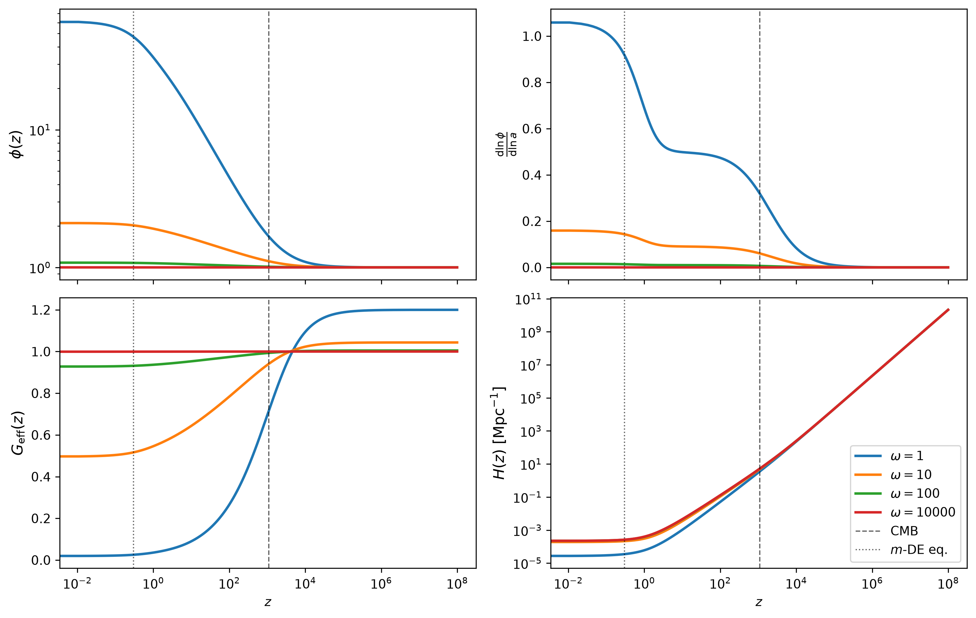
Figure 1: Field evolution for the Brans-Dicke theory with different values of $\omega$. Computed using the hi-class code in this tutorial notebook.
Now, Brans-Dicke theory can even be extended to cosmological scales, by setting the field in an expanding FLRW metric. When doing so, the Friedmann equation becomes:
\[\boxed{H^2 = \frac{8\pi \overline{\rho}}{3\phi} - \frac{K}{a^2}- H \frac{\dot{\phi}}{\phi} + \frac{\omega}{6}\frac{\dot{\phi}^2}{\phi^2}}\]It thus acquires three modifications compared to the standard form: i) $\dfrac{8\pi\overline\rho}{3\phi}$ instead of $\dfrac{8\pi G\overline\rho}{3}$ — the expected replacement $G \to 1/\phi$, now time-dependent. ii) $-H\dfrac{\dot\phi}{\phi}$ — a friction-like cross term between the expansion and the field, of indefinite sign. It has no analogue for a minimally coupled scalar and comes entirely from the non-minimal coupling. iii) $+\dfrac{\omega}{6}\dfrac{\dot\phi^2}{\phi^2}$ — the field’s own kinetic energy density, positive for $\omega>0$.
And the Klein-Gordon equation in a FLRW metric becomes:
\[\boxed{\ddot{\phi} + 3H \dot{\phi}= 8\pi \frac{\overline{\rho}-3\overline{P}}{2\omega + 3}}\]It is exactly the Klein–Gordon equation with Hubble friction $3H\dot\phi$ that we met for quintessence, but with $-\partial V/\partial\phi$ replaced by a source $\propto(\overline\rho - 3\overline P)$. The field is massless — there is no potential — and it is driven purely by matter. As for quintessence there are multiple ways to derive this equation: the simplest and most general being to replace $g$ by the FLRW metric in the equation of motion derived from the Lagrangian (above).
For completeness, the $ij$ component gives the acceleration equation
\[2\dot H + 3H^2 + \frac{K}{a^2} = -\frac{8\pi \overline{P}}{\phi} - \frac{\omega}{2}\frac{\dot\phi^2}{\phi^2} - \frac{\ddot\phi}{\phi} - 2H\frac{\dot\phi}{\phi},\]and — this is important — because $\nabla^\mu T_{\mu\nu}=0$ holds exactly (see the proof above), the continuity equation is completely unchanged from GR:
\[\dot{\overline{\rho}} + 3H\left(\overline{\rho}+\overline{P}\right) = 0 .\]So matter dilutes exactly as it always did, $\overline\rho \propto a^{-3(1+w)}$. Everything Brans-Dicke modifies is in how the expansion responds to that matter, never in the matter itself. However, as you might have guessed, the opposite conclusion would have been reached when working in the Einstein frame. For a discussion see also Barrow (1993).
Proof
geometry. For the FLRW metric, the Einstein tensor components are the standard ones,
\[G_{00} = 3\left(H^2 + \frac{K}{a^2}\right), \qquad G_{ij} = -\left(2\dot H + 3H^2 + \frac{K}{a^2}\right)g_{ij},\]with $H \equiv \dot a/a$. The matter components are $T_{00} = \overline\rho$, $T_{ij} = \overline P\,g_{ij}$, and the trace is
\[\mathcal{T} = g^{\mu\nu}T_{\mu\nu} = -\overline\rho + 3\overline P .\]All these relations are derived in our cosmology lecture.
derivatives of the field. Since $\phi=\phi(t)$ (we assume homoegeneity when considering only the background level), we have $\nabla_\mu\phi = (\dot\phi,0,0,0)$ and
\[(\nabla\phi)^2 = g^{00}\dot\phi^2 = -\dot\phi^2 .\]For the second derivatives, remember that $\nabla_\mu\nabla_\nu\phi = \partial_\mu\partial_\nu\phi - \Gamma^\lambda_{\mu\nu}\partial_\lambda\phi$ — the Christoffel piece is what makes the following non-trivial. In comoving coordinates \(\Gamma^\lambda_{00}=0\) and \(\Gamma^0_{ij} = H g_{ij}\), so
\[\nabla_0\nabla_0\phi = \ddot\phi, \qquad \nabla_i\nabla_j\phi = -H\,g_{ij}\,\dot\phi,\]and
\[\Box\phi = \frac{1}{\sqrt{-\vert g\vert}}\partial_\mu\!\left(\sqrt{-\vert g\vert}\,g^{\mu\nu}\partial_\nu\phi\right) = -\frac{1}{a^3}\frac{d}{dt}\!\left(a^3\dot\phi\right) = -\left(\ddot\phi + 3H\dot\phi\right).\]The $00$ equation. Evaluate the right-hand side of the field equation
\[G_{\mu\nu} = \frac{8\pi}{\phi}T_{\mu\nu} + \frac{\omega}{\phi^2}\left(\nabla_\mu\phi\nabla_\nu\phi - \tfrac12 g_{\mu\nu}(\nabla\phi)^2\right) + \frac{1}{\phi}\left(\nabla_\mu\nabla_\nu\phi - g_{\mu\nu}\Box\phi\right)\]component by component, with $g_{00}=-1$:
- kinetic bracket: $\;\dot\phi^2 - \tfrac12(-1)(-\dot\phi^2) = \dot\phi^2 - \tfrac12\dot\phi^2 = \tfrac12\dot\phi^2$;
- non-minimal bracket: $\;\ddot\phi - (-1)\left[-(\ddot\phi+3H\dot\phi)\right] = \ddot\phi - \ddot\phi - 3H\dot\phi = -3H\dot\phi$.
Notice the cancellation of $\ddot\phi$ — this is why the Friedmann equation, unlike the acceleration equation, contains only first derivatives of $\phi$. It remains a constraint equation, exactly as in GR. Therefore
\[3\left(H^2+\frac{K}{a^2}\right) = \frac{8\pi\overline\rho}{\phi} + \frac{\omega}{2}\frac{\dot\phi^2}{\phi^2} - 3H\frac{\dot\phi}{\phi},\]and dividing by $3$ and isolating $H^2$ gives the boxed Friedmann equation.
The $ij$ equation. Same exercise with $\nabla_i\nabla_j\phi = -Hg_{ij}\dot\phi$ and $T_{ij}=\overline P g_{ij}$:
- kinetic bracket: $\;0 - \tfrac12 g_{ij}(-\dot\phi^2) = \tfrac12 g_{ij}\dot\phi^2$;
- non-minimal bracket: $\;-Hg_{ij}\dot\phi + g_{ij}(\ddot\phi + 3H\dot\phi) = g_{ij}(\ddot\phi + 2H\dot\phi)$.
Every term is proportional to $g_{ij}$, as isotropy requires. Equating to $G_{ij} = -(2\dot H+3H^2+K/a^2)g_{ij}$ and cancelling $g_{ij}$ gives the acceleration equation.
The Klein-Gordon equation. Insert the derivative of the field into $\Box\phi = \dfrac{8\pi}{3+2\omega}\mathcal{T}$:
\[-\left(\ddot\phi + 3H\dot\phi\right) = \frac{8\pi\left(-\overline\rho+3\overline P\right)}{3+2\omega} \quad\Longrightarrow\quad \ddot\phi + 3H\dot\phi = \frac{8\pi\left(\overline\rho-3\overline P\right)}{3+2\omega},\]the two minus signs cancelling. Dividing by $\phi$ gives the boxed equation.
The cosmological evolution of the Brans-Dicke field is displayed on Figure 1 with the associated tutorial notebook to rederive the plot analytically or using the hi-class software. Let’s see if we can understand what is going on.
Early in the universe, during radiation dominated era, $\overline P = \overline\rho/3$, so $\mathcal{T} = -\overline\rho + 3\overline P = 0$ and the scalar equation becomes source-free:
\[\ddot\phi + 3H\dot\phi = 0 \quad\Longrightarrow\quad \dot\phi \propto a^{-3}.\]The field is not driven at all during radiation domination: its velocity redshifts away as $a^{-3}$ and $\phi$ rapidly freezes to a constant, so that $a\propto t^{1/2}$ exactly as in GR. This is the cosmological version of the statement in the previous section that the Brans-Dicke scalar is blind to radiation, and it has a practical consequence: primordial nucleosynthesis takes place with an essentially constant $G$, so BBN constrains the value of $G$ at that epoch rather than its rate of change.
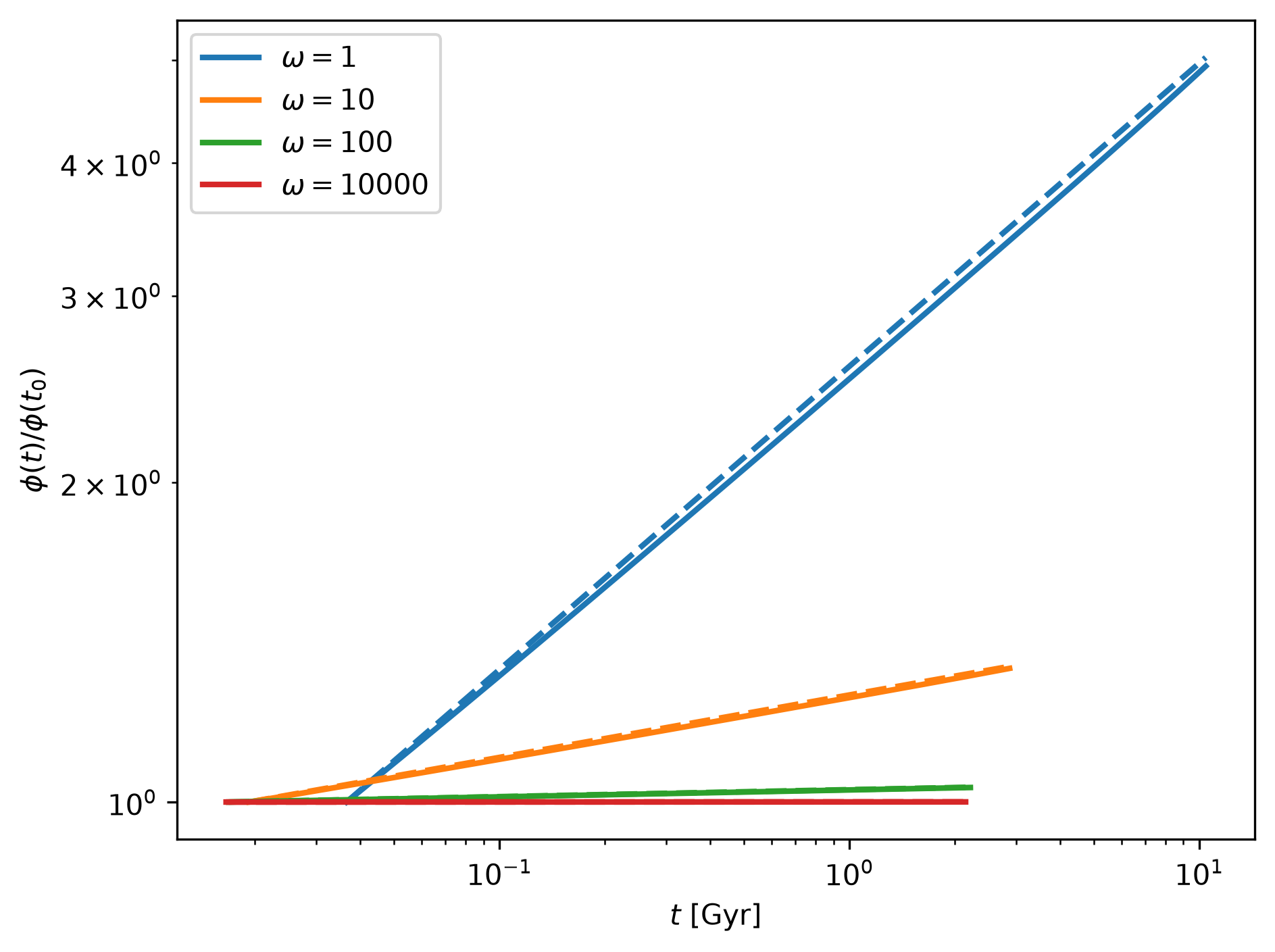
Figure 2: Power-law approximation during matter era. Comparaison with the the hi-class code in this tutorial notebook.
Later on, matter dominates. For a flat universe ($K=0$) filled with dust ($\overline P=0$), the system admits the exact power-law solution (Brans & Dicke 1961):
\[\boxed{a(t) \propto t^{\frac{2+2\omega}{4+3\omega}},\qquad \phi(t)\propto t^{\frac{2}{4+3\omega}}}\]Since $G_{\rm eff}\propto 1/\phi$, this solution yields an exact prediction:
\[\frac{\dot G}{G} = -\frac{\dot\phi}{\phi} = -\frac{2}{(4+3\omega)\,t} = -\frac{H}{1+\omega} .\]The last equality uses $t = \frac{2+2\omega}{4+3\omega}H^{-1}$ and is worth noting: the drift of $G$ is the Hubble rate, diluted by $\omega$.
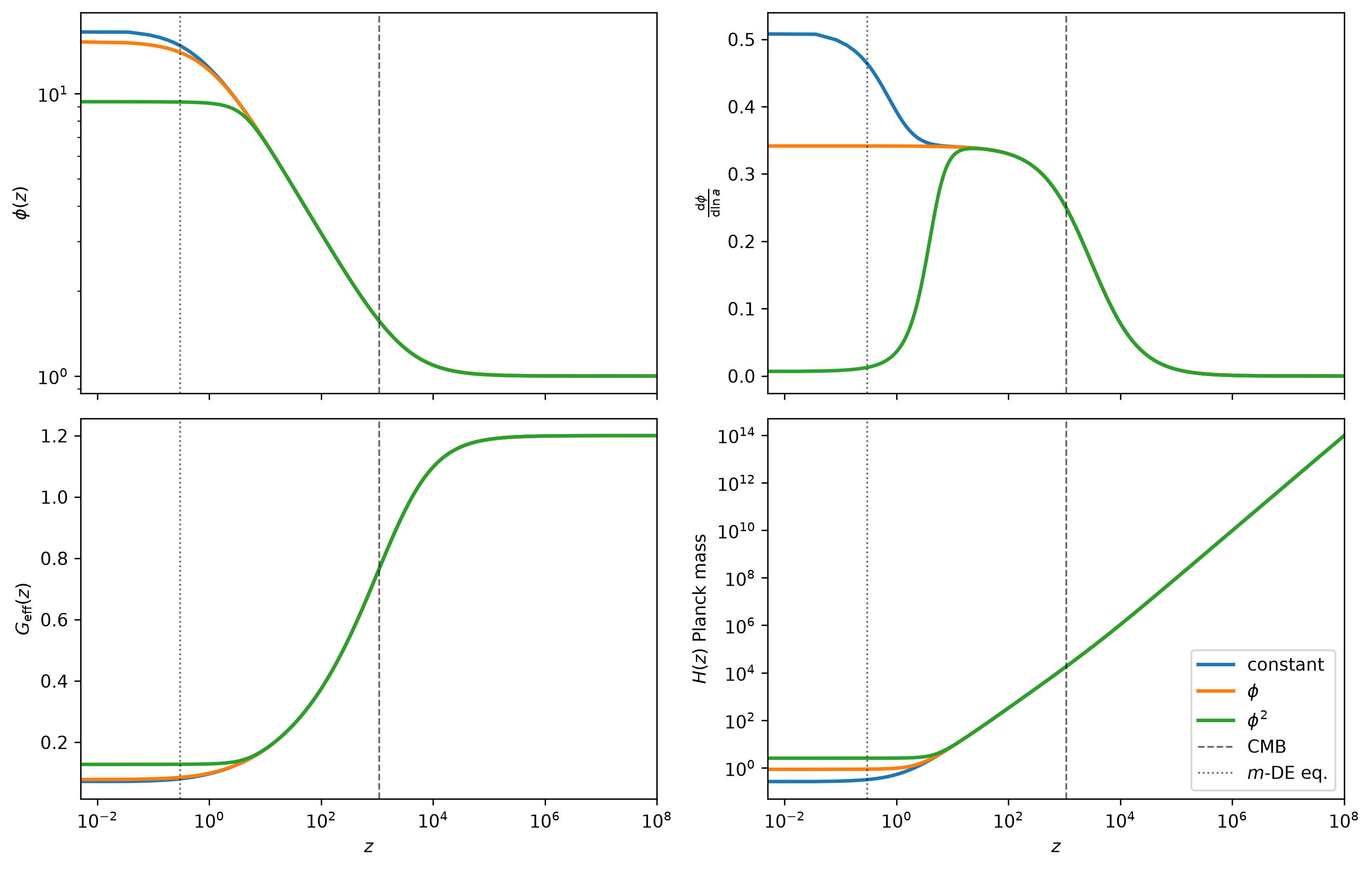
Figure 3: Analytical solution of Brans-Dicke cosmology with different potentials. Computed by integration with scipy in this tutorial notebook.
We see that while the field seems to have reached a plateau today, its velocity is non zero, and is actually maximal. The field will continue evolving along with dark energy. The exact evolution depends on how exactly dark energy is implemented (as discussed above). If the field has a potential $V(\phi)$, the two cosmological equations become:
\[H^2 = \frac{8\pi \overline{\rho}}{3\phi} - H \frac{\dot{\phi}}{\phi} + \frac{\omega}{6}\frac{\dot{\phi}^2}{\phi^2} + \frac{8\pi}{3} \frac{V(\phi)}{\phi}\] \[\ddot{\phi} + 3H \dot{\phi}= \frac{8\pi}{2\omega + 3}\Bigg(\overline{\rho}-3\overline{P} + 4V(\phi) - 2\frac{\text{d}V}{\text{d}\ln(\phi)}\Bigg)\]The field evolution for the three potentials discussed as “roads to dark energy” $V_0, V_0\phi$ and $V_0\phi^2$ are displayed on Figure 3.
Proof
With a potential, the Lagrangian is simply:
\[\boxed{\mathcal{L} = \frac{1}{16\pi}\left(\phi R - \frac{\omega}{\phi}g^{\mu\nu}\partial_\mu\phi\,\partial_\nu\phi\right) - V(\phi) + \mathcal{L}_{m}[\psi,g],}\]The experimental constraints on Brans-Dicke theory
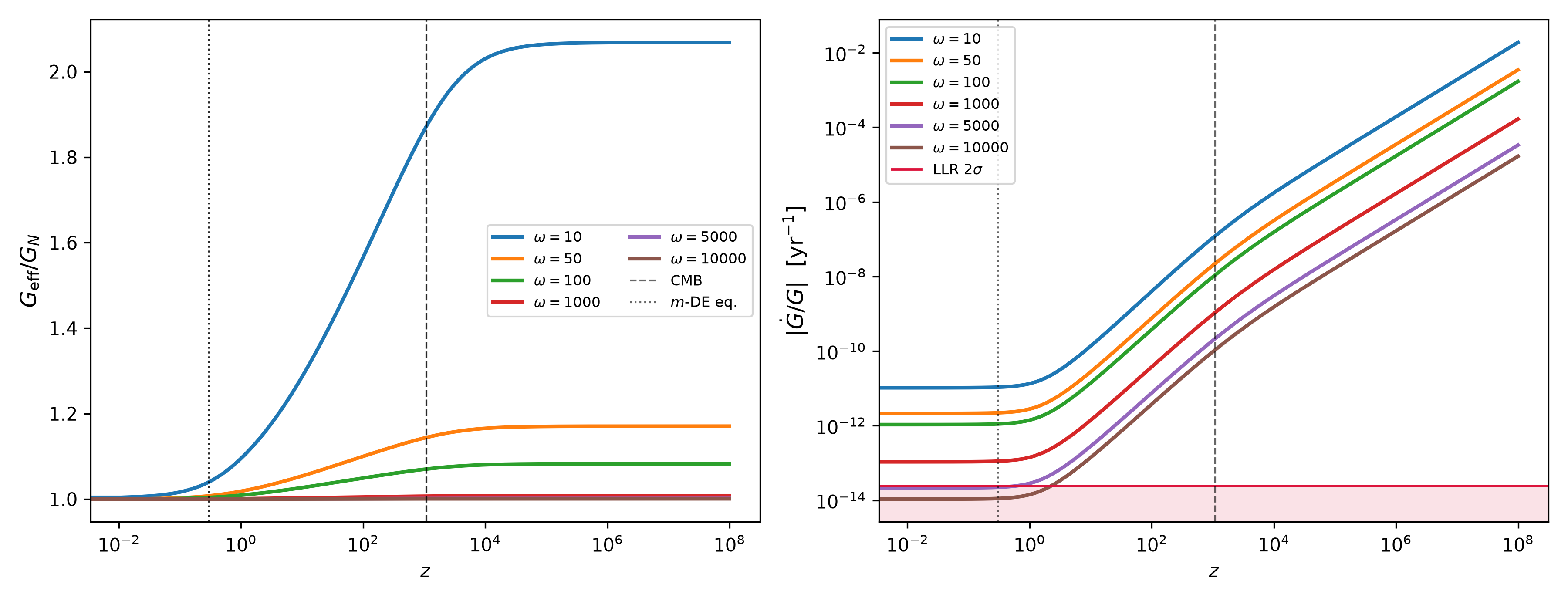
Figure 4: Illustration of the constraints on $\omega$ by LLR. Using hi-class in the tutorial notebook.
The PPN parameters for Brans-Dicke theory are:
\[\boxed{\;G_{\rm eff} = \frac{1}{\phi_0}\cdot\frac{2\omega+4}{2\omega+3}\;}\qquad\qquad \boxed{\;\gamma = \frac{1+\omega}{2+\omega}\;}\]\(G_{\rm eff}\) corresponds directly to the $\mu$ parameter defined in our cosmology class, while $\Sigma=0$ for this model (as it does not couple to light).
Three different $G$ in Brans-Dicke!
You might think that $G=1/\phi$, after all this is the whole raison d’être of this theory! This is true at the Lagrangian level, so at the “fundamental level” per say, but this $G$ is not what would be measured as $G$ if one were to consider two masses attracted by gravity (e.g. a Cavendish experiment). The second is what we could call the effective coupling constant $G_{\rm eff}$.
Consider the weak field limit of the theory. Take $g_{\mu\nu} = \eta_{\mu\nu} + h_{\mu\nu}$ and $\phi = \phi_0 + \varphi$, with $\vert h_{\mu\nu}\vert\ll1$ and $\vert\varphi\vert\ll\phi_0$, around a static point source of mass $M$ ($T_{00}=\rho$, $T_{ij}=0$, $T = -\rho$).
First, linearize the field equation of motion $\partial_\mu\partial^\mu\phi = 8\pi\mathcal{T}/(3+2\omega)$ for a static configuration, $\nabla^2\varphi = -\dfrac{8\pi\rho}{3+2\omega}$. With $\nabla^2(1/r) = -4\pi\delta^{(3)}$,
\[\varphi(r) = \frac{2}{3+2\omega}\,\frac{M}{r}\]You might then think that $G = \dfrac{2}{3+2\omega}$. Still not right! $\varphi$ here is the Brans-Dicke field, it is not the total gravitational potential felt by an object. If you want, this is the $\varphi$ component of the gravitational force. To it, one must add the gravitational field of the standard GR metric!
The proper way to find $G_{\rm eff}$ is to use the Einstein equations, containing also the field $\phi$, to find the $00$ component of the metric as
\[g_{00} = - 1 + \frac{2 G_{\rm eff}M}{c^2r}\]Now, at linear order most terms drop in the Einstein equation (the $\omega\,\partial\phi\partial\phi/\phi^2$ pieces are quadratic in $\varphi$) and what remains is
\[G^{(1)}_{\mu\nu}[h] = \frac{8\pi}{\phi_0}T_{\mu\nu} + \frac{1}{\phi_0}\Big(\partial_\mu\partial_\nu\varphi - \eta_{\mu\nu}\partial_\alpha\partial^\alpha\varphi\Big).\]Reading $g_{00}$ off is easier from the Ricci form. Taking the trace (\(G^{(1)}=-R^{(1)}\), \(\eta^{\mu\nu}\eta_{\mu\nu}=4\)) and using the scalar equation \(\Box\varphi = 8\pi \mathcal{T}/(3+2\omega)\):
\[G^{(1)} = \frac{8\pi \mathcal{T}}{\phi_0} - \frac{3\,\Box\varphi}{\phi_0} = \frac{8\pi \mathcal{T}}{\phi_0}\left(1-\frac{3}{3+2\omega}\right) = \frac{8\pi \mathcal{T}}{\phi_0}\,\frac{2\omega}{3+2\omega}.\]Substituting into \(R^{(1)}_{\mu\nu} = G^{(1)}_{\mu\nu} - \tfrac12\eta_{\mu\nu}G^{(1)}\), the two $\eta_{\mu\nu}\mathcal{T}$ contributions combine as $\frac{1}{3+2\omega}+\frac{\omega}{3+2\omega}=\frac{1+\omega}{3+2\omega}$, leaving the compact form
\[\boxed{\;R^{(1)}_{\mu\nu} = \frac{8\pi}{\phi_0}\left(T_{\mu\nu} - \frac{1+\omega}{3+2\omega}\,\eta_{\mu\nu}T\right) + \frac{1}{\phi_0}\,\partial_\mu\partial_\nu\varphi\;}\]Notice what happened: the $\varphi$ source is no longer a trace term, and the coefficient of $\eta_{\mu\nu}T$ is no longer the GR value $\tfrac12$. That shift from $\tfrac12$ to $\frac{1+\omega}{3+2\omega}$ is the whole effect.
Considering the $00$ component. Write \(g_{00}=-(1-2U)\), \(g_{ij}=(1+2\gamma U)\delta_{ij}\) with \(U=G_{\rm eff}M/r\), so that \(R^{(1)}_{00}=-\nabla^2U\). For a static source \(\partial_0\partial_0\varphi=0\), and with $T_{00}=\rho$, $\eta_{00}=-1$, $T=-\rho$:
\[T_{00} - \frac{1+\omega}{3+2\omega}\eta_{00}\mathcal{T} = \rho\left(1-\frac{1+\omega}{3+2\omega}\right) = \rho\,\frac{2+\omega}{3+2\omega}.\]So \(-\nabla^2U = \dfrac{8\pi\rho}{\phi_0}\dfrac{2+\omega}{3+2\omega}\), and comparing with Newton, \(\nabla^2 U = -4\pi G_{\rm eff}\rho\):
\[\boxed{\;G_{\rm eff} = \frac{1}{\phi_0}\,\frac{2\omega+4}{2\omega+3}\;}\]The three $G$’s. Now we can name them:
| value | what measures it | |
|---|---|---|
| $G_{\rm bare} = 1/\phi$ | Lagrangian coupling | nothing directly |
| $\dfrac{2}{3+2\omega}$ | scalar exchange alone | nothing — it is only half the story |
| $G_{\rm eff} = \dfrac{1}{\phi}\dfrac{2\omega+4}{2\omega+3}$ | Cavendish | two masses attracting |
The middle entry is exactly the piece the naive reasoning stops at, and one can see it inside the third: writing $\frac{2\omega+4}{2\omega+3} = 1 + \frac{1}{2\omega+3}$,
\[G_{\rm eff} = \underbrace{\frac{1}{\phi}}_{\text{tensor exchange}} + \underbrace{\frac{1}{\phi}\frac{1}{2\omega+3}}_{\text{scalar exchange}}\]Gravity in Brans-Dicke is the sum of two forces: the usual graviton, plus a scalar. As $\omega\to\infty$ the scalar piece dies as $1/2\omega$ and we recover general relativity.
And there is a fourth twist, which we prove in the next box: the $G$ that light feels is not $G_{\rm eff}$ but the bare $1/\phi$. The scalar pulls on matter and not on light — which is precisely why lensing is such a clean way to test these theories.
$\gamma$ in Brans-Dicke
$\gamma$ is obtained from the $jk$ Einstein equation. With $T_{ij}=0$, $\eta_{ij}=\delta_{ij}$ and $T=-\rho$, the boxed Ricci equation of the previous box gives
\[R^{(1)}_{ij} = \frac{8\pi\rho}{\phi_0}\,\frac{1+\omega}{3+2\omega}\,\delta_{ij} \;+\; \frac{1}{\phi_0}\,\partial_i\partial_j\varphi .\]For the static metric \(g_{00}=-(1-2U)\), $g_{ij}=(1+2\gamma U)\delta_{ij}$ one computes the linearized Ricci tensor from \(R^{(1)}_{\mu\nu}=\tfrac12\left(-\Box h_{\mu\nu}-\partial_\mu\partial_\nu h+\partial_\mu\partial^\alpha h_{\alpha\nu}+\partial_\nu\partial^\alpha h_{\alpha\mu}\right)\), with \(h=2U(3\gamma-1)\), giving
\[R^{(1)}_{ij} = -\gamma\,\delta_{ij}\nabla^2 U \;+\; (1-\gamma)\,\partial_i\partial_j U .\]The equation therefore splits into two independent pieces, and each one determines $\gamma$ on its own — a useful consistency check.
(i) The $\partial_i\partial_j$ part. Matching the traceless structures,
\[(1-\gamma)\,U = \frac{\varphi}{\phi_0} \qquad\Longrightarrow\qquad (1-\gamma)\,\frac{G_{\rm eff}M}{r} = \frac{1}{\phi_0}\frac{2M}{(3+2\omega)r}.\]Inserting $G_{\rm eff}=\frac{1}{\phi_0}\frac{2\omega+4}{2\omega+3}$, the $\phi_0$ and $(2\omega+3)$ cancel and
\[(1-\gamma)(2\omega+4) = 2 \qquad\Longrightarrow\qquad 1-\gamma = \frac{1}{\omega+2}.\](ii) The $\delta_{ij}$ part. Using $\nabla^2U=-4\pi G_{\rm eff}\rho$,
\[4\pi\gamma\,G_{\rm eff}\,\rho = \frac{8\pi\rho}{\phi_0}\frac{1+\omega}{3+2\omega} \qquad\Longrightarrow\qquad \gamma\,(2\omega+4) = 2(1+\omega).\]Both routes give the same answer:
\[\boxed{\;\gamma = \frac{\omega+1}{\omega+2} = 1 - \frac{1}{\omega+2}\;}\]Why this is the interesting number. $\gamma$ measures how much space curvature is produced per unit mass — equivalently the ratio $\Phi/\Psi$ of the two metric potentials. In GR $\gamma=1$ exactly. Any deviation is gravitational slip, and it is the cleanest signature that something other than a spin-2 field is mediating the force. It is also what Cassini measured to $\gamma-1 = (2.1\pm2.3)\times10^{-5}$, giving $\omega\gtrsim4\times10^4$.
And now the fourth $G$. Light does not respond to $\Psi$ alone but to the combination $\Phi+\Psi$, i.e. to $G_{\rm eff}(1+\gamma)/2$. Substituting,
\[G_{\rm light} = \frac{G_{\rm eff}(1+\gamma)}{2} = \frac{1}{2\phi_0}\,\frac{2\omega+4}{2\omega+3}\cdot\frac{2\omega+3}{\omega+2} = \frac{1}{\phi_0}.\]Exactly the bare Lagrangian value. The scalar-exchange enhancement that appears in $G_{\rm eff}$ cancels precisely against the deficit in $\gamma$. Physically: a massless scalar carries no helicity-2 component, so it can pull on matter but cannot bend light — photons are conformally invariant and blind to it.
This is the origin of the statement, used repeatedly in later lectures, that in Brans-Dicke
\[\mu = \frac{1}{\phi}\frac{2\omega+4}{2\omega+3}, \qquad \gamma = \frac{\omega+1}{\omega+2}, \qquad \Sigma = \frac{\mu(1+\gamma)}{2} = \frac{1}{\phi} \;\;\textbf{exactly.}\]Now, the Brans-Dicke model has to face the very sharp observational constraints in the following table:
| quantity | Brans–Dicke prediction | measurement |
|---|---|---|
| $\gamma - 1$ | $-\dfrac{1}{2+\omega}$ | $(2.1\pm2.3)\times10^{-5}$ (Cassini) → $\omega > 4\times10^4$ |
| Nordtvedt parameter $\eta_N = 4\beta-\gamma-3$ | $\dfrac{1}{2+\omega}$ | $\vert \eta_N \vert < 3\times10^{-4}$ (LLR) |
| $\dot G/G$ (matter era) | $\sim -\dfrac{2}{(3\omega+4)\,t}\;\sim\;-\dfrac{H_0}{\omega}$ | $\vert \dot G /G \vert = (-5.0 \pm 9.6)\times 10^{-15}$ yr$^{-1}$ (LLR) |
Sources: see previous lecture.
The evolution of $G$ and $\dot{G}$ for the Brans-Dicke model is displayed on Figure 4 for different values of $\omega$. We see that the LLR bound alone already forces $\omega \gtrsim 5\times 10^3$, and the Cassini bound on $\gamma$ is stronger still, $\omega > 4\times10^4$. A proper constraint on $\omega$ would of course require sampling this local data together with cosmological data. This can be done using a MCMC sampler as Cobaya or MontePython and implementing the LLR bounds as Gaussian likelihoods.
We can now finally ask whether the theory still does what it was built for: is $\phi$ — hence $1/G$ — fixed by the matter content of the universe?
Suppose it were entirely so. The scalar equation $\Box\phi = 8\pi\mathcal{T}/(3+2\omega)$ is linear, so its solution splits as $\phi = \phi_{\rm matter} + \phi_{\rm hom}$, with $\phi_{\rm matter}$ the piece sourced by matter (retarded Green’s function) and $\phi_{\rm hom}$ the source-free piece, fixed by boundary and initial data alone. The Machian hypothesis is $\phi_{\rm hom}=0$, and in the static weak-field limit it gives
\[\phi_{\rm matter} \;=\; \frac{2}{(3+2\omega)c^2}\sum_k \frac{m_k}{r_k} \;\simeq\; \frac{2}{3+2\omega}\frac{\mathfrak{M}}{Rc^2}\]for a universe of mass $\mathfrak{M}$ and radius $R$. Inserting this into $G_{\rm eff}$ above, the theory would then predict
\[\chi \equiv \frac{G_{\rm eff}\mathfrak{M}}{Rc^2} = \frac{2\omega+4}{2} = \omega + 2 .\]But $\chi$ is not ours to choose: we estimated it in the Mach section from observation, $\chi \simeq \Omega_{\rm tot}/2 \simeq 0.5$. A purely matter-sourced $\phi$ is therefore compatible with our universe only for $\omega = \mathcal{O}(1)$ — Dicke’s own preferred value, and four orders of magnitude below what Cassini allows.
Turned around: keeping the observed $\chi$ and the measured $\omega$, the matter-sourced fraction of the field is
\[\frac{\phi_{\rm matter}}{\phi_{\rm total}} \;=\; \frac{\chi}{\omega+2} \;\simeq\; \frac{1}{\omega+2} \;\lesssim\; 2\times10^{-5}.\]Less than 0.003% of the gravitational coupling is Machian in origin. The other 99.997% is $\phi_{\rm hom}$ — boundary data, not matter: precisely the “absolute element” that Mach wanted to eliminate, and that we already found sitting inside GR.
And the trade-off is structural, not accidental: every deviation from GR in the table above scales as $1/\omega$, so the large-$\omega$ limit that rescues the theory from the $\gamma$ and $\dot G$ bounds is the very same limit that annihilates its Machian content. Brans-Dicke is Machian only in the regime where it is excluded, and GR is simply its perfectly non-Machian endpoint $\omega\to\infty$.
General scalar tensor theories
Conformally coupled scalars
Brans–Dicke theory can be straightforwardly generalized by letting the three functions of $\phi$ be arbitrary:
\[S_{\rm ST} = \frac{1}{16\pi G_0}\int \sqrt{\vert-g\vert}\left[\, F(\phi)R - Z(\phi)\, g^{\mu\nu}\partial_\mu\phi\partial_\nu\phi - 2U(\phi) \,\right]d^4x + S_m[g_{\mu\nu},\psi]\]- $F(\phi)$ = non-minimal coupling function, dimensionless; $G_0/F$ is the effective, $\phi$-dependent Newton “constant”. Pulling the constant $G_0$ out front is what makes $F$ dimensionless — this is the convention of Esposito-Farèse & Polarski, and it is the one that keeps every formula below free of stray powers of $G_0$. Because $G$ varies, this is again a theory violating SEP.
- $Z(\phi)$ = kinetic normalization (dimensionless).
- $U(\phi)$ = potential (a $\phi$-dependent cosmological term), of dimension $[\,\text{length}\,]^{-2}$. The choice $V(\phi)=2U(\phi)$ is a convention commonly used in the litterature.
- $\psi$ = collective notation for all matter fields; $S_m$ depends on $\phi$ only through $g_{\mu\nu}$ — this is the statement of the weak equivalence principle (and EEP) in the Jordan frame. This is again still a metric theory of gravity.
Theories with such actions are known as scalar–tensor theories. Brans–Dicke is the special case $F=\phi$, $Z=\omega/\phi$, $U=0$ (if one normalizes the action by today’s cosmological value of the field \(G_0= 1/\phi_0\)). Two conditions must hold for such a theory to be healthy: $F>0$ (positive graviton kinetic energy, i.e. gravity is attractive) and $3F’^2+2ZF>0$ (no ghost in the scalar sector — see the dedicated discussion below). For Brans-Dicke, they are $\phi >0$ and $3 + 2\omega >0$ that is $\omega > -3/2$ which was already a condition that we identified earlier!
Einstein-frame
Now, as for Brans–Dicke, we consider the conformal transformation of the metric, keeping the same convention as above ($\Omega$ for the rescaling towards the Einstein frame, $A=\Omega^{-1}$ for the matter coupling):
\[\tilde g_{\mu\nu} = F(\phi)\,g_{\mu\nu} \equiv \Omega^2g_{\mu\nu}, \qquad \Omega^2 = F, \qquad A^2 \equiv \Omega^{-2} = \frac{1}{F}\](a pointwise rescaling of the metric — it preserves angles and causal structure but not lengths as long as $F>0$), as well as a redefinition of the scalar so that its kinetic term takes the canonical form $-\tfrac12(\partial\tilde\phi)^2$:
\[\boxed{\;\left(\frac{\text{d}\tilde\phi}{\text{d}\phi}\right)^{2} \;=\; M_{\rm Pl}^{2}\,\frac{3F'^{2}+2ZF}{2F^{2}}\;},\qquad F'\equiv\frac{\text{d}F}{\text{d}\phi}.\]where we introduced the reduced Planck mass \(M_{\rm Pl} \equiv \frac{1}{\sqrt{8\pi G_0}} \qquad (\hbar=c=1)\). The canonical field $\tilde\phi$ has the dimensions of a mass, like any ordinary scalar in field theory.
Then, the equation of a general scalar-tensor theory takes the following form in the Einstein frame:
\[S = \int d^4x\,\sqrt{-\vert \tilde g\vert}\left[\frac{M_{\rm Pl}^{2}}{2}\tilde R \;-\; \frac12\,\tilde g^{\mu\nu}\partial_\mu\tilde\phi\,\partial_\nu\tilde\phi \;-\; V(\tilde\phi)\right] \;+\; S_m\!\left[A^{2}(\tilde\phi)\,\tilde g_{\mu\nu},\,\psi\right]\]where we introduced the comonly used notations:
\[V = \frac{M_{\rm Pl}^{2}\,U}{F^{2}} \;=\; \frac{U}{8\pi G_0 F^{2}}.\]This is exactly the Einstein–Hilbert action ($\frac{M_{\rm Pl}^2}{2}\tilde R = \frac{\tilde R}{16\pi G_0}$) plus a textbook minimally coupled scalar with a potential. Everything non-standard has been pushed into the argument of $S_m$. The Jordan/Einstein frame transformation is not a feature of Brans-Dicke theory, it is thus much more general.
Proof
Write $\tilde g_{\mu\nu}=\Omega^2 g_{\mu\nu}$ with $\Omega^2 = F$. In four dimensions we already encountered multiple times the required ingredients which are
\[\sqrt{-\vert g\vert} = \Omega^{-4}\sqrt{-\vert \tilde g\vert} = F^{-2}\sqrt{-\vert \tilde g\vert},\qquad g^{\mu\nu} = \Omega^{2}\tilde g^{\mu\nu} = F\,\tilde g^{\mu\nu},\] \[R = \Omega^{2}\Big[\tilde R + 6\,\tilde\Box\ln \Omega - 6\,\tilde g^{\mu\nu}\partial_\mu\ln \Omega\,\partial_\nu\ln \Omega\Big].\]The curvature term. With $\ln \Omega=\tfrac12\ln F$,
\[\sqrt{-\vert g\vert}\,F R = F^{-2}\sqrt{-\vert \tilde g\vert}\cdot F\cdot F\Big[\tilde R + 3\tilde\Box\ln F - \tfrac32(\tilde\nabla\ln F)^2\Big] = \sqrt{-\vert \tilde g\vert}\Big[\tilde R + 3\tilde\Box\ln F - \tfrac32\frac{(\tilde\nabla F)^2}{F^{2}}\Big].\]The two factors of $F$ cancel against $F^{-2}$ — this is the whole point of choosing $\Omega^2=F$. The $\tilde\Box\ln F$ term is a total derivative and integrates away.
The kinetic term.
\[-\sqrt{-\vert g\vert}\,Z\,g^{\mu\nu}\partial_\mu\phi\partial_\nu\phi = -F^{-2}\sqrt{-\vert \tilde g\vert}\cdot Z\cdot F\,\tilde g^{\mu\nu}\partial_\mu\phi\partial_\nu\phi = -\sqrt{-\vert \tilde g\vert}\;\frac{Z}{F}\,(\tilde\nabla\phi)^2 .\]The potential. $-2\sqrt{-\vert g\vert}\,U = -\sqrt{-\vert \tilde g\vert}\;\dfrac{2U}{F^{2}}$.
Collecting, and using $\partial_\mu F = F’\partial_\mu\phi$:
\[S = \frac{1}{16\pi G_0}\int d^4x\,\sqrt{-\vert \tilde g\vert}\left[\tilde R - \left(\frac{3}{2}\frac{F'^2}{F^2}+\frac{Z}{F}\right)(\tilde\nabla\phi)^2 - \frac{2U}{F^2}\right] + S_m[F^{-1}\tilde g,\psi],\]where $F^{-1}\tilde g_{\mu\nu} = A^2\tilde g_{\mu\nu}$ is indeed the Jordan (matter) metric. Note that the kinetic coefficient is $\dfrac{3F’^2+2ZF}{2F^2}$ — hence the no-ghost condition $3F’^2+2ZF>0$ (ensuring that the kinetic energy of the field is positive) quoted above.
Canonical normalisation. Substitute $\dfrac{1}{16\pi G_0}=\dfrac{M_{\rm Pl}^2}{2}$ and demand that the scalar piece equal $-\tfrac12(\tilde\nabla\tilde\phi)^2$:
\[\frac{M_{\rm Pl}^{2}}{2}\cdot\frac{3F'^{2}+2ZF}{2F^{2}}\,(\tilde\nabla\phi)^{2} \;\stackrel{!}{=}\; \frac{1}{2}\left(\frac{\text{d}\tilde\phi}{\text{d}\phi}\right)^{2}(\tilde\nabla\phi)^{2} \quad\Longrightarrow\quad \left(\frac{\text{d}\tilde\phi}{\text{d}\phi}\right)^{2} = M_{\rm Pl}^{2}\,\frac{3F'^{2}+2ZF}{2F^{2}}.\]The same substitution in the potential gives $\dfrac{M_{\rm Pl}^{2}}{2}\cdot\dfrac{2U}{F^{2}} = \dfrac{M_{\rm Pl}^{2}U}{F^{2}} \equiv V$.
For Brans–Dicke normalized by \(G_0=1/\phi_0\), $F= \phi$, $Z=\omega/\phi$ give $\left(\text{d}\tilde\phi/\text{d}\phi\right)^2=M_{\rm Pl}^2(2\omega+3)/2\phi^2$, hence after integration:
\[\tilde\phi = M_{\rm Pl}\sqrt{\frac{2\omega+3}{2}}\;\ln\phi ,\]the same logarithm we already met in the Brans–Dicke lecture, now carrying an explicit factor of $M_{\rm Pl}$ so that $\tilde\phi$ has mass dimension one.
Deviation from GR
In this frame, gravity is thus (again) a pure Einstein with a minimally coupled canonical scalar, and all the modification hides in the matter coupling function \(A(\tilde\phi)\) which tells us which metric matter actually feels. The key observable is the logarithmic slope of $A$, made dimensionless with $M_{\rm Pl}$:
\[\boxed{\;\beta(\tilde\phi) \;\equiv\; M_{\rm Pl}\,\frac{\text{d}\ln A}{\text{d}\tilde\phi} \;=\; -\,M_{\rm Pl}\,\frac{\text{d}\ln \Omega}{\text{d}\tilde\phi}\;}\]— the strength of the scalar force relative to gravity. Equivalently, a constant $\beta$ means $A(\tilde\phi)=e^{\beta\tilde\phi/M_{\rm Pl}}$, the exponential coupling, which appears all over the place in the screening literature.
One can show that the field equation in the Einstein frame is
\[\tilde\Box\tilde\phi = \frac{\text{d}V}{\text{d}\tilde\phi} \;-\; \frac{\beta(\tilde\phi)}{M_{\rm Pl}}\,\tilde{\mathcal T},\]where $\tilde{\mathcal T}\equiv\tilde g_{\mu\nu}\tilde T^{\mu\nu}$ is the trace of the Einstein-frame stress tensor $\tilde T^{\mu\nu}\equiv\frac{2}{\sqrt{-\vert \tilde g\vert}}\frac{\delta S_m}{\delta \tilde g_{\mu\nu}}$. In the static limit around a point mass $\tilde M$ with $V=0$,
\[\tilde\phi(r) = -\,\frac{\beta\,\tilde M}{4\pi M_{\rm Pl}\,r}, \qquad \vec a = -\frac{G_0\tilde M}{r^{2}}\big(1+2\beta^{2}\big)\,\hat r, \qquad \boxed{\;\frac{F_{\tilde\phi}}{F_N} = 2\beta^{2}\;}\]Proof
The field equation. Vary the Einstein-frame action with respect to $\tilde\phi$.
Scalar part. $-\tfrac12(\partial\tilde\phi)^2 - V$ gives, after one integration by parts, $\sqrt{-\vert \tilde g\vert}\left[\tilde\Box\tilde\phi - V’(\tilde\phi)\right]\delta\tilde\phi$.
Matter part. $S_m$ depends on $\tilde\phi$ only through the matter metric $g_{\mu\nu}=A^2\tilde g_{\mu\nu}$, so with $T^{\mu\nu}=\frac{2}{\sqrt{-\vert g\vert}}\frac{\delta S_m}{\delta g_{\mu\nu}}$,
\[\frac{\delta S_m}{\delta\tilde\phi} = \frac{\delta S_m}{\delta g_{\mu\nu}}\,\frac{\partial g_{\mu\nu}}{\partial\tilde\phi} = \frac{\sqrt{-\vert g\vert}}{2}T^{\mu\nu}\cdot 2A\frac{\text{d}A}{\text{d}\tilde\phi}\,\tilde g_{\mu\nu}.\]Using $\tilde g_{\mu\nu}=A^{-2}g_{\mu\nu}$, $\sqrt{-\vert g\vert}=A^{4}\sqrt{-\vert \tilde g\vert}$ and $\tilde{\mathcal T}=A^{4}\mathcal T$ (with $\mathcal T = g_{\mu\nu}T^{\mu\nu}$), everything collapses:
\[\frac{\delta S_m}{\delta\tilde\phi} = \sqrt{-\vert \tilde g\vert}\,A^{3}\frac{\text{d}A}{\text{d}\tilde\phi}\,\mathcal T = \sqrt{-\vert \tilde g\vert}\,\frac{\text{d}\ln A}{\text{d}\tilde\phi}\,\tilde{\mathcal T} = \sqrt{-\vert \tilde g\vert}\,\frac{\beta}{M_{\rm Pl}}\,\tilde{\mathcal T}.\]Adding the two pieces and setting the total to zero,
\[\tilde\Box\tilde\phi = \frac{\text{d}V}{\text{d}\tilde\phi} - \frac{\beta}{M_{\rm Pl}}\tilde{\mathcal T}.\]The scalar is sourced by the trace — so radiation ($\mathcal T=0$) does not source it, exactly as in Brans–Dicke and Nordstrom theories.
Static limit. For dust $\tilde{\mathcal T}=-\tilde\rho$, so $\nabla^{2}\tilde\phi = \dfrac{\beta}{M_{\rm Pl}}\tilde\rho$, and for a point mass
\[\tilde\phi(r) = -\frac{\beta\tilde M}{4\pi M_{\rm Pl}\,r}.\]Again, same as for Nordstrom and Brans-Dicke before: In the Einstein frame a test particle has action $S=-m\int\text{d}s = -m\int A(\tilde\phi)\text{d}\tilde s$: its mass depends on $\tilde\phi$. In the non-relativistic limit it therefore feels the potential $\ln A$ in addition to the metric potential $\Phi=-G_0\tilde M/r$:
\[\vec a = -\nabla\Phi - \nabla\ln A = -\nabla\Phi - \frac{\beta}{M_{\rm Pl}}\nabla\tilde\phi = -\frac{G_0\tilde M}{r^2}\hat r - \frac{\beta^{2}\tilde M}{4\pi M_{\rm Pl}^{2}r^{2}}\hat r .\]The last step uses $M_{\rm Pl}^{-2}=8\pi G_0$, so that $\dfrac{\beta^2}{4\pi M_{\rm Pl}^2}=2\beta^2 G_0$. Both terms are attractive, and we can read off the equation that
\[G_{\rm eff} = G_0\big(1+2\beta^{2}\big).\]The effective gravitational constant measured by a Cavendish like experiment is thus:
\[G_{\rm eff} = G_0\big(1+2\beta^{2}\big).\]For Brans–Dicke. $A=\phi^{-1/2}$ (and $\Omega = \phi^{1/2}$) and $\text{d}\tilde\phi/\text{d}\phi=M_{\rm Pl}\sqrt{(2\omega+3)/2}\,/\phi$ give
\[\beta = M_{\rm Pl}\,\frac{\text{d}\ln A/\text{d}\phi}{\text{d}\tilde\phi/\text{d}\phi} = \frac{-1/2}{\sqrt{(2\omega+3)/2}} = -\frac{1}{\sqrt{2(2\omega+3)}},\]so $2\beta^2 = 1/(2\omega+3)$ and
\[G_{\rm eff} = G_0\left(1+\frac{1}{2\omega+3}\right) = G_0\,\frac{2\omega+4}{2\omega+3}\]which is precisely what we derived previously. This is a nice generalisation of Nordström and Brans–Dicke theories. For Brans–Dicke, $2\beta^2 = 1/(2\omega+3)$ = const; in particular metric $f(R)$ gravity, which as we will see is Brans–Dicke with $\omega=0$, gives $\beta=-1/\sqrt6$ and the famous $G_{\rm eff}=\tfrac43 G_0$.
Disformal couplings
The conformal map $g_{\mu\nu}=A^2(\phi)\tilde g_{\mu\nu}$ between the gravity metric $\tilde g$ and the metric $g$ that matter feels is not the most general relation one can build from $\phi$ and $\tilde g$. Bekenstein (1992) showed that one may also add a piece along $\partial_\mu\phi$:
\[g_{\mu\nu} = A^{2}(\phi,X)\,\tilde g_{\mu\nu} \;+\; B(\phi,X)\,\partial_\mu \phi\,\partial_\nu\phi , \qquad X \equiv -\tfrac12 \tilde g^{\mu\nu}\partial_\mu\phi\partial_\nu\phi\]Note the second term carries its indices from the two gradients — there is no extra $\tilde g_{\mu\nu}$. The difference is physical, not cosmetic:
- the conformal piece rescales all directions equally, so it preserves angles and light cones;
- the disformal piece singles out the direction $\partial_\mu\phi$, so it stretches time relative to space along the scalar’s gradient. Light cones in the two frames no longer coincide, and photons and matter can propagate at different speeds.
Causality requires $A^2>0$ and $A^2 - 2XB > 0$; the second condition is what keeps $g$ Lorentzian (it is the factor appearing in $\det g = A^{8}\left(1-2XB/A^{2}\right)\det\tilde g$, and it is where the sign convention for $X$ matters: with the opposite convention $X\to-X$ one finds the familiar $A^2+2XB>0$).
Two facts make this more than a curiosity:
- $B=B(\phi)$ functions are part of Horndeski theories discussed in the dedicated class it just moves you around inside the same theory space.
- $B=B(\phi,X)$ takes you outside Horndeski theories, into beyond-Horndeski / DHOST theories. This is the cleanest constructive way to generate healthy higher-derivative theories: apply a disformal map to a Horndeski theory and the result has higher-order equations of motion but no Ostrogradsky ghost, because it is secretly a field redefinition of a healthy theory.
Disformal couplings are also how one evades GW170817 while keeping structure: since photons follow $g_{\mu\nu}$ and gravitons $\tilde g_{\mu\nu}$, the constraint $c_T=c$ becomes a condition on $B$. We will not discuss this in detail here.
Pathological theories: Ghosts, instabilities and tachyons
General considerations
As we saw, not all values of the functions $F,Z,U$ give a healthy theory. As a general matter of fact, when facing a modified gravity theory one should always check for pathological behaviour: ghosts, gradient instabilities and tachyons. The first two are fatal, and arise in many simple modified gravity theories.
The general method is always the same: perturb the theory at linear order around a background (FLRW, if you are a cosmologist), keep the action to second order in the perturbation $\delta$, and go to Fourier space. Whatever the theory, the result takes the general form
\[\mathcal A\,\omega^{2} = \mathcal B\,\frac{k^{2}}{a^{2}} + \mathcal C,\]with three background-dependent coefficients $\mathcal A$ (kinetic), $\mathcal B$ (gradient) and $\mathcal C$ (mass). Dividing by $\mathcal A$, this is the classical wave dispersion relation already met for gravitational waves,
\[\omega^{2} = c_s^{2}\,\frac{k^{2}}{a^{2}} + m^{2},\]with \(c_s^{2} \equiv \frac{\mathcal B}{\mathcal A}\) and \(\;m^{2} \equiv \frac{\mathcal C}{\mathcal A}\) where $c_s$ is the speed of sound — really the propagation speed of the perturbation, in units of $c$ — and $m$ its effective mass. Note that only the ratios are physical, but the signs of $\mathcal B$ and $\mathcal A$ separately are what must be checked: flipping both leaves $c_s^2>0$ while making the mode a ghost.
Three coefficients, three ways to be sick:
-
$\mathcal A<0$ is a ghost: the kinetic term has the wrong sign, so the mode’s energy is unbounded from below. Fatal. On its own a ghost is harmless (an overall sign on a decoupled action changes nothing), but as soon as it couples to a healthy sector — and gravity couples everything — the vacuum can decay into (ghost quanta of energy $-E$) + (photons or particles of energy $+E$) for any $E$.
-
$c_s^{2}<0$ is a gradient instability: $\omega=\pm i\vert c_s\vert k/a$, so every mode grows as $e^{\vert c_s\vert kt/a}$. Also fatal — and classically so, no quantum argument needed: the growth rate is proportional to $k$, so the shorter the wavelength the faster the blow-up, and no cutoff can be low enough to save the background.
-
$m^{2}<0$ is a tachyon: modes grow as $e^{\vert m\vert t}$, at a rate independent of $k$. Usually benign — it just means you expanded around a maximum of the potential. This is ordinary symmetry breaking; it is also the Jeans instability, which built every galaxy. It only matters when $\vert m\vert$ greatly exceeds the relevant background rate ($H$ in cosmology) with no nearby minimum to fall into.
The decisive difference is the $k$-dependence of the growth rate. Ghosts and gradient instabilities get worse at short wavelength, so no effective description survives; a tachyon does not.
How to do in practice
A way to inspect the sanity of a theory is to first go to the Einstein frame, then expand the action at second order in $\delta \phi$ and read the value of the coefficients $\mathcal{A}$, $\mathcal{B}$ and $\mathcal{C}$. The reason this works is because perturbations really are second order in the action, once the first order has been cancelled to find the equations of motion.
What follows is inspired by Alessandra Silvestri lectures, and we refer to them for more details. Concretely, we split the field into a homogeneous background plus a small perturbation,
\[\phi(t,\vec{x}) = \bar{\phi}(t) + \delta\phi(t,\vec{x}),\]on a flat FLRW metric $ds^2 = -dt^2 + a^2(t)\,\delta_{ij}dx^i dx^j$, with $H \equiv \dot{a}/a$ and signature $(-,+,+,+)$. Expanding the action gives
\[S = \underbrace{S_0[\bar\phi]}_{\text{background}} + \underbrace{S_1[\bar\phi]\,\delta\phi}_{=\,0\ \text{by the background e.o.m.}} + \;S_2[\delta\phi] + \mathcal{O}(\delta\phi^3),\]so $S_2$ is the leading object controlling the perturbations. The target is always to bring it to the form
\[S_2 = \frac{1}{2}\int dt\,d^3x\;a^3\left[\;\mathcal{A}\,\dot{\delta\phi}^{\,2}\;-\;\mathcal{B}\,\frac{(\partial_i\delta\phi)^2}{a^2}\;-\;\mathcal{C}\,\delta\phi^2\;\right],\]where the three coefficients \(\mathcal{A},\mathcal{B}$ and $\mathcal{C}\) correspond to the coefficients discussed in the previous section, allowing to identify the presence of pathologies.
For a general field Lagrangian in the Einstein frame
\[\mathcal{L}(\phi,X), \qquad X = -\frac{1}{2}\partial_\mu \phi\, \partial^\mu\phi\]where $X$ is the canonical kinetic term (on the background, $\bar{X}=\tfrac12\dot{\bar\phi}^2$), the second order expansion is
\[S_2 = \frac{1}{2}\int dt\,d^3x\;a^3\left[\left(\mathcal{L}_{,X}+2X\mathcal{L}_{,XX}\right)\dot{\delta\phi}^{\,2}\;-\;\mathcal{L}_{,X}\,\frac{(\partial_i\delta\phi)^2}{a^2}\;-\;\left(\frac{1}{a^3}\frac{d}{dt}\!\left(a^3\,\mathcal{L}_{,\phi X}\,\dot{\bar\phi}\right)-\mathcal{L}_{,\phi\phi}\right)\delta\phi^2\right]\]with the shorthand \(\mathcal{L}_{,X}\equiv\partial\mathcal{L}/\partial X\), \(\mathcal{L}_{,\phi}\equiv\partial\mathcal{L}/\partial\phi\), and bars dropped from here on.
Proof
First, expand $X$ itself. This is the only place the gradient term is born:
\[X = \frac{1}{2}\left(\dot{\bar\phi}+\dot{\delta\phi}\right)^2 - \frac{1}{2a^2}(\partial_i\delta\phi)^2 = \bar{X} + \underbrace{\dot{\bar\phi}\,\dot{\delta\phi}}_{\delta X^{(1)}} + \underbrace{\frac{1}{2}\dot{\delta\phi}^{\,2} - \frac{1}{2a^2}(\partial_i\delta\phi)^2}_{\delta X^{(2)}}\]Note that $\delta X^{(1)}$ contains only a time derivative: the background is homogeneous, so a spatial gradient can only appear squared, i.e. at second order. This single fact is why $\mathcal{A}\neq\mathcal{B}$ is possible at all.
Taylor expand $\mathcal{L}$ to second order in the two variables $\delta\phi$ and $\delta X$:
\[\mathcal{L} = \bar{\mathcal{L}} + \mathcal{L}_{,\phi}\,\delta\phi + \mathcal{L}_{,X}\,\delta X + \frac{1}{2}\mathcal{L}_{,\phi\phi}\,\delta\phi^2 + \mathcal{L}_{,\phi X}\,\delta\phi\,\delta X + \frac{1}{2}\mathcal{L}_{,XX}\,(\delta X)^2 + \dots\]Collect everything of second order. There are exactly four contributions:
\[\mathcal{L}_{,X}\,\delta X^{(2)} = \frac{1}{2}\mathcal{L}_{,X}\dot{\delta\phi}^{\,2} - \frac{1}{2}\mathcal{L}_{,X}\frac{(\partial_i\delta\phi)^2}{a^2}\] \[\frac{1}{2}\mathcal{L}_{,XX}\left(\delta X^{(1)}\right)^2 = \frac{1}{2}\mathcal{L}_{,XX}\,\dot\phi^2\,\dot{\delta\phi}^{\,2} = \frac{1}{2}\left(2X\mathcal{L}_{,XX}\right)\dot{\delta\phi}^{\,2}\qquad(\text{using }\dot\phi^2=2X)\] \[\mathcal{L}_{,\phi X}\,\delta\phi\,\delta X^{(1)} = \mathcal{L}_{,\phi X}\,\dot\phi\;\delta\phi\,\dot{\delta\phi}, \qquad\qquad \frac{1}{2}\mathcal{L}_{,\phi\phi}\,\delta\phi^2\]The first two combine into the \(\dot{\delta\phi}^2\) coefficient \(\mathcal{L}_{,X}+2X\mathcal{L}_{,XX}\), while only the first supplies a gradient term.
Kill the cross term by parts. Writing $\delta\phi\,\dot{\delta\phi} = \tfrac{1}{2}\tfrac{d}{dt}(\delta\phi^2)$ and integrating by parts inside $\int dt\,d^3x\,a^3$:
\[\int dt\,d^3x\;a^3\,\mathcal{L}_{,\phi X}\dot\phi\;\frac{1}{2}\frac{d}{dt}\!\left(\delta\phi^2\right) = -\frac{1}{2}\int dt\,d^3x\;a^3\left[\frac{1}{a^3}\frac{d}{dt}\!\left(a^3\mathcal{L}_{,\phi X}\dot\phi\right)\right]\delta\phi^2\]which is the second piece of $\mathcal{C}$. Assembling the four terms gives $S_2$ above.
From this, we read:
\[\mathcal{A} = \mathcal{L}_{,X} + 2X\,\mathcal{L}_{,XX}, \qquad \mathcal{B} = \mathcal{L}_{,X},\] \[c_s^2 = \frac{\mathcal{B}}{\mathcal{A}} = \frac{\mathcal{L}_{,X}}{\mathcal{L}_{,X}+2X\mathcal{L}_{,XX}}, \qquad m^2 = \frac{\mathcal{C}}{\mathcal{A}} = \frac{\dfrac{1}{a^3}\dfrac{d}{dt}\!\left(a^3\mathcal{L}_{,\phi X}\dot\phi\right)-\mathcal{L}_{,\phi\phi}}{\mathcal{L}_{,X}+2X\mathcal{L}_{,XX}}\]so that a theory is healthy provided
\[\mathcal{L}_{,X}+2X\mathcal{L}_{,XX} > 0 \quad\text{(no ghost)} \qquad\text{and}\qquad \mathcal{L}_{,X} > 0 \quad\text{(no gradient instability)} .\]Two remarks:
- The ghost condition involves $\mathcal{L}_{,XX}$, the gradient one does not. A theory linear in $X$ can never have a gradient instability — you need a genuinely non-linear kinetic function to make $\mathcal{A}$ and $\mathcal{B}$ disagree.
- The sign of $\mathcal{A}$ is only meaningful relative to the graviton, whose kinetic term is fixed positive by the Einstein-frame term $+\tfrac{1}{2}M_{\rm Pl}^2 R$. This is precisely why we go to the Einstein frame first: it removes the kinetic mixing between $\phi$ and the metric that makes the Jordan-frame signs unreadable.
- $\mathcal{A}$ and $\mathcal{B}$ are unaffected by metric perturbations (those only shift $\mathcal{C}$ by a term $\sim -\frac{1}{a^3}\frac{d}{dt}\big(a^3\dot\phi^2/M_{\rm Pl}^2H\big)$), so the “test field” expansion above is enough for the ghost and gradient verdicts.
For quintessence, Brans–Dicke and scalar–tensor we get:
| theory | Einstein-frame $\mathcal{L}(\phi,X)$ | $\mathcal{A}$ | $c_s^2$ | $m^2$ | verdict |
|---|---|---|---|---|---|
| Quintessence | $X - V(\phi)$ | $1$ | $1$ | $V_{,\phi\phi}$ | always healthy |
| Brans–Dicke | \(\dfrac{(2\omega_{\rm BD}+3)M_{\rm Pl}^2}{2\phi^2}\,X - \tilde{V}(\phi)\) | \(\dfrac{(2\omega_{\rm BD}+3)M_{\rm Pl}^2}{2\phi^2}\) | $1$ | \(\tilde V_{,\tilde{\phi}\tilde{\phi}}\) | ghost iff \(\omega_{\rm BD}<-\tfrac{3}{2}\) |
| Scalar–tensor | \(\dfrac{M_{\rm Pl}^2\!\left(2F\omega+3F_{,\phi}^2\right)}{2F^2}\,X - \dfrac{M_{\rm Pl}^4 V}{F^2}\) | \(\dfrac{M_{\rm Pl}^2\!\left(2F\omega+3F_{,\phi}^2\right)}{2F^2}\) | $1$ | \(\tilde V_{,\tilde{\phi}\tilde{\phi}}\) | ghost iff \(2F\omega+3F_{,\phi}^2<0\) |
| k-essence | \(\mathcal{L}(\phi,X)\) | \(\mathcal{L}_{,X}+2X\mathcal{L}_{,XX}\) | \(\dfrac{\mathcal{L}_{,X}}{\mathcal{L}_{,X}+2X\mathcal{L}_{,XX}}\) | see above | both are possible |
The first three rows all have $c_s^2=1$ exactly. This is not a coincidence: they are all linear in $X$, and a conformal transformation preserves light cones, so a unit propagation speed in one frame is a unit propagation speed in the other. Gradient instabilities simply do not occur in this class — you have to leave it (k-essence, or Horndeski) to get $c_s^2\neq1$.
General stress energy tensor
Note that in such a general framework, varying $S=\int d^4x\sqrt{-\vert g\vert}\,\mathcal{L}(\phi,X)$ with respect to the metric,
\[T_{\mu\nu} = -\frac{2}{\sqrt{-\vert g\vert}}\frac{\delta\!\left(\sqrt{-\vert g\vert}\,\mathcal{L}\right)}{\delta g^{\mu\nu}} = \mathcal{L}_{,X}\,\partial_\mu\phi\,\partial_\nu\phi + g_{\mu\nu}\,\mathcal{L}\]which is exactly the perfect-fluid form $T_{\mu\nu}=(\rho_\phi+p_\phi)u_\mu u_\nu + p_\phi\, g_{\mu\nu}$ once we identify the four-velocity with the (normalised) gradient of the field,
\[u_\mu = -\frac{\partial_\mu\phi}{\sqrt{2X}}, \qquad u^\mu u_\mu = -1 ,\]giving
\[p_\phi = \mathcal{L}, \qquad \rho_\phi = 2X\mathcal{L}_{,X} - \mathcal{L}, \qquad \rho_\phi + p_\phi = 2X\,\mathcal{L}_{,X} .\]A useful consistency check: the fluid sound speed computed thermodynamically at fixed $\phi$ reproduces the one read off from $S_2$,
\[\left.\frac{\partial p_\phi}{\partial\rho_\phi}\right|_\phi = \frac{\mathcal{L}_{,X}}{\mathcal{L}_{,X}+2X\mathcal{L}_{,XX}} = c_s^2 .\]and hence
\[1+w_\phi = \frac{\rho_\phi+p_\phi}{\rho_\phi} = \frac{2X\,\mathcal{L}_{,X}}{2X\mathcal{L}_{,X}-\mathcal{L}} = \frac{2X\,\mathcal{L}_{,X}}{\rho_\phi} .\]For quintessence ($\mathcal{L}=X-V$) this is just $1+w_\phi = \dot\phi^2/\left(\tfrac12\dot\phi^2+V\right)\ \geq 0$.
The general formula makes the link between the equation of state and stability explicit. Since \(\mathcal{B}=\mathcal{L}_{,X}\), and assuming $X>0$ and $\rho_\phi>0$,
\[\mathrm{sign}\left(1+w_\phi\right) = \mathrm{sign}\left(\mathcal{L}_{,X}\right) = \mathrm{sign}\left(\mathcal{B}\right) .\]So a phantom equation of state $w_\phi<-1$ forces $\mathcal{B}<0$, and therefore either a ghost ($\mathcal{A}<0$) or a gradient instability ($c_s^2<0$). This is the standard no-go: a single scalar field with a Lagrangian of the form $\mathcal{L}(\phi,X)$, minimally coupled to gravity, cannot cross the phantom divide $w_\phi=-1$ without becoming unstable.
Further reading and watching
- Barbour & Pfister - From Newton’s Bucket to Quantum Gravity - 1995
- T. Baker - Modified gravity & dark energy - Youtube lectures
- Brans, C. & Dicke, R. H. (1961), Mach’s principle and a relativistic theory of gravitation, Phys. Rev. 124, 925.
- Alessandra Silvestri: “Dark Energy and Modified Gravity” - Youtube videos
-
Recall however as we saw in the field lecture, that the EEP can be forced on us from field theoretical arguments about possible couplings of a spin-2 field with matter. ↩