f(R) gravity

Overview: adding higher orders

So far, every theory we met went beyond GR by adding a field: a scalar in Brans-Dicke, four free functions of a scalar in Horndeski, a vector in generalised Proca, a mass for the graviton. All of these break assumption L2 of Lovelock’s theorem (“the metric is the only field”) and W9 of Weinberg-Deser (“no other light fields coupling to matter”).

In this class we attack a different assumption: L3, “the field equations are of at most second order in derivatives” (equivalently W6, “two derivatives only”). The idea is disarmingly simple. The Einstein-Hilbert Lagrangian is linear in the Ricci scalar $R$. Why should Nature stop at first order? Why not

\[\mathcal{L} \;\propto\; R \;+\; \alpha R^2 \;+\; \beta R^3 \;+\;\dots \;\equiv\; f(R)\ ?\]

This is the road sketched in Figure 1, and the family of theories obtained this way is called $f(R)$ gravity. It is by far the most studied modified gravity theory after Brans-Dicke — partly because it is easy to write down, partly because, as we will discover, it is secretly a theory we already know.

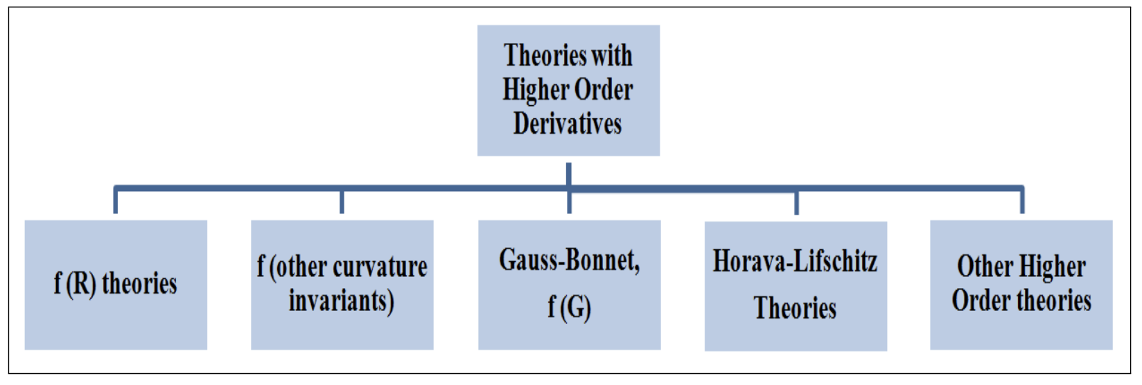
Figure 1: A roadmap of higher-order models of modified gravity. Credit: Ishak et al. (2024).

Historically, the idea is old: Buchdahl (1970) already studied non-linear Lagrangians in cosmology (MNRAS 150, 1), and Starobinsky (1980) used $f(R)=R+R^2/6M^2$ to build the first working model of inflation (Phys. Lett. B 91, 99). The modern wave of interest started when Carroll, Duvvuri, Trodden & Turner (2004) proposed $f(R)=R-\mu^4/R$ as an explanation of cosmic acceleration without dark energy — a proposal which, as we shall see, died within months.

A warning before we start: Ostrogradsky’s theorem

There is a very good reason why almost nobody adds higher derivatives lightly. Let us state the danger precisely, since it will control everything below.

Ostrogradsky’s theorem (1850). If a Lagrangian $L(q,\dot q,\ddot q,\dots)$ depends on derivatives higher than the first, and is non-degenerate in its highest derivative (i.e. $\partial^2 L/\partial\ddot q^{\,2}\neq0$ can be solved for $\ddot q$), then the corresponding Hamiltonian is linear in at least one canonical momentum, and is therefore unbounded from below.

Definitions. A ghost is a degree of freedom whose kinetic energy has the wrong sign, so that its energy is unbounded from below. This is not merely “unstable”: in a theory containing both a ghost and an ordinary field, the vacuum can decay into ghost + ordinary particle pairs at no energy cost, with a phase-space volume that diverges. Degenerate means that the highest-derivative terms are not independent, so the Legendre transform to the Hamiltonian is not invertible and Ostrogradsky’s construction does not apply.

Two remarks that will matter:

A generic higher-curvature theory, say $\mathcal{L}=R+aR^2+bR_{\mu\nu}R^{\mu\nu}$, does propagate an Ostrogradsky ghost: it carries $2$ (massless graviton) $+\,1$ (scalar) $+\,5$ (massive spin-2) $=8$ modes, and the massive spin-2 has negative kinetic energy. This is Stelle gravity (Stelle 1977) — remarkably, it is perturbatively renormalizable, and that renormalizability is bought precisely with the ghost.
$f(R)$ is the exception. Because $R$ contains second derivatives of the metric only linearly (this was the whole content of the “$g^{\mu\nu}\delta R_{\mu\nu}$ is a total divergence” statement we proved in the Brans-Dicke class), the theory is degenerate. Its field equations are fourth order, but they propagate only $2+1=3$ healthy modes. The one extra mode is a scalar, and we will meet it in a moment under the name scalaron.

For a very readable modern account of the theorem and its loopholes, see Woodard (2015).

The theory

We take the action

\[\boxed{\;S = \frac{1}{16\pi G}\int \text{d}^4x\,\sqrt{-\vert g\vert}\;f(R) \;+\; S_m[g_{\mu\nu},\psi]\;}\]

where $f$ is an arbitrary function, $G$ is a bare constant (we will see below that it is not what a Cavendish experiment measures — exactly the same subtlety as the three $G$’s of Brans-Dicke), and $\psi$ collectively denotes matter fields. Note that matter couples to $g_{\mu\nu}$ and to nothing else: $f(R)$ gravity is a metric theory, it satisfies the WEP and the EEP by construction, and it will violate the SEP. Setting $f(R)=R-2\Lambda$ recovers GR with a cosmological constant.

We write throughout

\[f_R \equiv \frac{\text{d}f}{\text{d}R},\qquad f_{RR}\equiv\frac{\text{d}^2f}{\text{d}R^2}.\]

Varying with respect to the metric gives the field equations:

\[\boxed{\;f_R\,R_{\mu\nu} \;-\; \tfrac12 f\,g_{\mu\nu} \;+\; \big(g_{\mu\nu}\Box - \nabla_\mu\nabla_\nu\big)f_R \;=\; 8\pi G\,T_{\mu\nu}\;}\]

Proof

We need the same three ingredients as in the Brans-Dicke derivation:

$\delta\sqrt{-\vert g\vert} = -\tfrac12\sqrt{-\vert g\vert}\,g_{\mu\nu}\delta g^{\mu\nu}$ (proved in the first lecture);
$\delta R = R_{\mu\nu}\delta g^{\mu\nu} + g^{\mu\nu}\delta R_{\mu\nu}$;
$g^{\mu\nu}\delta R_{\mu\nu} = g_{\mu\nu}\Box\,\delta g^{\mu\nu} - \nabla_\mu\nabla_\nu\,\delta g^{\mu\nu}$, which we established in the Brans-Dicke class by showing that $g^{\mu\nu}\delta R_{\mu\nu}=\nabla_\rho v^\rho$ is a pure divergence.

Then

\[\delta\big(\sqrt{-\vert g\vert}f\big) = \sqrt{-\vert g\vert}\left[f_R\,\delta R - \tfrac12 f g_{\mu\nu}\delta g^{\mu\nu}\right] = \sqrt{-\vert g\vert}\left[\Big(f_R R_{\mu\nu} - \tfrac12 f g_{\mu\nu}\Big)\delta g^{\mu\nu} + f_R\,g^{\mu\nu}\delta R_{\mu\nu}\right].\]

This is the crucial step. In GR $f_R=1$ is constant, the last term is a total divergence, and it is discarded as a boundary term — which is exactly why Einstein’s equations are second order despite $R$ containing second derivatives. Here $f_R$ is a function of the metric, so the divergence is weighted by a non-constant factor and no longer integrates away. Instead we integrate by parts twice:

\[\int\sqrt{-\vert g\vert}\;f_R\left[g_{\mu\nu}\Box - \nabla_\mu\nabla_\nu\right]\delta g^{\mu\nu} = \int\sqrt{-\vert g\vert}\;\left[g_{\mu\nu}\Box f_R - \nabla_\mu\nabla_\nu f_R\right]\delta g^{\mu\nu}.\]

Each integration by parts moves one derivative from $\delta g^{\mu\nu}$ onto $f_R$, discarding a genuine boundary term. Adding the matter variation, with $T_{\mu\nu}\equiv-\frac{2}{\sqrt{-\vert g\vert}}\frac{\delta S_m}{\delta g^{\mu\nu}}$, gives the boxed result.

Where the fourth derivatives come from: $f_R$ already contains second derivatives of $g$ (through $R$), and $\Box f_R$ adds two more. Compare with the Brans-Dicke equations, where the identical structure $\nabla_\mu\nabla_\nu\phi - g_{\mu\nu}\Box\phi$ appeared — but with $\phi$ an independent field, so the equations stayed second order. The whole difference between $f(R)$ and Brans-Dicke is whether that scalar is independent or built out of the metric. Keep this in mind: it is the seed of the equivalence we prove below.

The scalaron

Take the trace of the field equations (contract with $g^{\mu\nu}$, using $g^{\mu\nu}g_{\mu\nu}=4$ and writing $T\equiv g^{\mu\nu}T_{\mu\nu}$):

\[\boxed{\;3\,\Box f_R \;+\; f_R R \;-\; 2f \;=\; 8\pi G\,T\;}\]

Stare at this equation, because it contains all the physics of the theory. In GR, $f=R$, $f_R=1$, and it reduces to $-R = 8\pi G T$: an algebraic relation, the Ricci scalar is slaved to the matter content instantaneously and locally. As soon as $f_{RR}\neq0$, the equation becomes a wave equation for $f_R$: the Ricci scalar acquires a life of its own. It can oscillate, propagate, carry energy and persist in vacuum.

This propagating mode is called the scalaron. It is the extra degree of freedom of $f(R)$ gravity, and everything that follows — fifth forces, screening, growth of structure, inflation — is a statement about it.

We can read off its dynamics by rewriting the trace equation as $3\Box f_R = \text{d}V_{\rm eff}/\text{d}f_R$ with

\[\frac{\text{d}V_{\rm eff}}{\text{d}f_R} \;=\; \frac{1}{3}\big(2f - f_R R + 8\pi G\,T\big),\]

and its mass is the curvature of this effective potential:

\[\boxed{\;m^2 \;=\; \frac13\left(\frac{f_R}{f_{RR}} - R\right)\;\simeq\;\frac{1}{3f_{RR}}\quad\text{when } \vert f_{RR}\vert R\ll f_R\simeq1.\;}\]

Two immediate consequences, both essential:

$f_{RR}>0$ is required. Otherwise $m^2<0$: the scalaron is a tachyon, and short-wavelength perturbations grow exponentially with a rate that diverges as $k\to\infty$. This is the Dolgov-Kawasaki instability (Dolgov & Kawasaki 2003), and it is what killed the $f(R)=R-\mu^4/R$ model of Carroll et al. within a year: for that model $f_{RR}=-6\mu^4/R^3<0$, and the instability timescale inside ordinary matter is $\sim10^{-26}$ s. Not a subtle problem.
The mass depends on $R$, hence on the local density. In a dense region $R$ is large, $f_{RR}$ is small, $m$ is large, and the scalaron force is short-ranged. This should ring a loud bell: it is exactly the chameleon mechanism of the screening class. We will make this identification exact below.

The associated length scale is the Compton wavelength of the scalaron, $\lambda_C \equiv 1/m \simeq \sqrt{3f_{RR}}$, and it is the single most important quantity in the phenomenology: the theory looks like GR on scales $\gg\lambda_C$ and is maximally modified on scales $\ll\lambda_C$.

$f(R)$ is Brans-Dicke in disguise

We now prove the statement we have been teasing since the Lovelock class.

$f(R)$ gravity with $f_{RR}\neq0$ is exactly equivalent to a Brans-Dicke theory with $\omega=0$ and a potential.

Note the logic carefully: we set out to break assumption L3 (higher derivatives) and we landed back on assumption L2 (extra field). This is remark 1 of the Lovelock class made concrete — almost every road to modified gravity collapses onto extra degrees of freedom.

Proof

Step 1 — introduce an auxiliary field. Consider the action

\[S = \frac{1}{16\pi G}\int \text{d}^4x\sqrt{-\vert g\vert}\;\Big[f(\chi) + f_\chi(\chi)\,(R-\chi)\Big] + S_m,\]

where $\chi$ is a new scalar field with no kinetic term at all and $f_\chi\equiv \text{d}f/\text{d}\chi$.

Step 2 — vary with respect to $\chi$. Since $\chi$ appears without derivatives, its equation of motion is purely algebraic:

\[f_\chi + f_{\chi\chi}(R-\chi) - f_\chi = f_{\chi\chi}\,(R-\chi) = 0 .\]

Provided $f_{\chi\chi}\neq0$, the unique solution is $\chi = R$. Substituting back, the action collapses to $\frac{1}{16\pi G}\int\sqrt{-\vert g\vert}f(R)$: the two actions are classically equivalent. (This is where the condition $f_{RR}\neq0$ earns its keep: if $f_{RR}=0$ then $f$ is linear, we are in GR, and $\chi$ is not determined.)

Step 3 — rename. Define

\[\phi \equiv f_\chi(\chi) = f_R, \qquad V(\phi) \equiv \chi(\phi)\,\phi - f\big(\chi(\phi)\big),\]

which is nothing but a Legendre transform of $f$ — the same operation that takes a Lagrangian to a Hamiltonian. The action becomes

\[\boxed{\;S = \frac{1}{16\pi G}\int \text{d}^4x\sqrt{-\vert g\vert}\;\Big[\phi R - V(\phi)\Big] + S_m[g_{\mu\nu},\psi]\;}\]

Step 4 — compare. Recall the Brans-Dicke Lagrangian from the dedicated class:

\[\mathcal{L}_{\rm BD} = \frac{1}{16\pi}\left(\phi_{\rm BD} R - \frac{\omega}{\phi_{\rm BD}}g^{\mu\nu}\partial_\mu\phi_{\rm BD}\partial_\nu\phi_{\rm BD}\right) + \mathcal{L}_m .\]

With the identification $\phi_{\rm BD} = \phi/G = f_R/G$ (our $\phi$ is dimensionless, theirs had the dimension of $1/G$), the two match provided $\omega=0$, with the addition of a potential $V$. $\blacksquare$

This is a beautiful and slightly deflating result. Beautiful, because a fourth-order theory of the metric alone has been traded for a second-order theory of a metric plus a scalar — Ostrogradsky is evaded not by luck but because the Legendre transform exists. Deflating, because we have not discovered a new road after all.

It also lets us import every result of the Brans-Dicke class for free. In particular, from the Horndeski table, $f(R)$ sits inside Horndeski with (beware of the notation clash: in that table the Horndeski scalar is called $\phi$ but plays the role of $R$, whereas the scalar we just built above is $\phi=f_R$ — the two are related by the Legendre transform, and one has to say which one is meant)

\[G_2 = -\frac{M_{\rm Pl}^2}{2}\big(\phi f'(\phi) - f(\phi)\big) = -\frac{M_{\rm Pl}^2}{2}V, \qquad G_4 = \frac{M_{\rm Pl}^2}{2}f'(\phi), \qquad G_3=G_5=0,\]

so that $\alpha_T=0$ identically and $\alpha_B = -\alpha_M$. $f(R)$ is a luminal Horndeski theory: gravitational waves travel at exactly $c$, and GW170817 — which annihilated so much of the Horndeski landscape — has nothing to say about it. That is one of the reasons $f(R)$ is still so widely used as a benchmark: it is one of the few survivors.

Palatini $f(R)$: a different theory with the same name

A parenthesis worth making, because it is a classic source of confusion. In the Palatini formulation one varies the metric and the connection independently. For GR this changes nothing: the connection equation forces $\Gamma$ to be Levi-Civita. For $f(R)$ it changes everything: the connection turns out to be the Levi-Civita connection of the conformally rescaled metric $f_R\,g_{\mu\nu}$, and the resulting theory is equivalent to Brans-Dicke with

\[\omega = -\frac32 .\]

We met this value before: it is exactly the boundary at which the scalar’s kinetic term $\propto(2\omega+3)$ vanishes. The scalaron is therefore not dynamical in Palatini $f(R)$ — its value is fixed algebraically by the trace $T$ of the matter stress tensor. Consequences:

no propagating extra mode, hence no fifth force in vacuum, hence trivial solar-system tests;
but the metric now depends algebraically on the local matter density and its derivatives. This produces curvature singularities at the surface of polytropic stars (Barausse, Sotiriou & Miller 2008) and unacceptable corrections to atomic physics — the hydrogen spectrum itself is modified (Olmo 2008).

Metric $f(R)$ and Palatini $f(R)$ are two genuinely different physical theories built from the same function $f$. Everything else in this class refers to the metric version.

The Einstein frame and the chameleon

Apply now the machinery of the Brans-Dicke class: perform the conformal transformation $\tilde g_{\mu\nu} = F(\phi)g_{\mu\nu}$ with $F=\phi=f_R$, and canonically normalise. Using the general scalar-tensor formulas established there, with $F=\phi$, $Z=0$, $2U=V$:

\[\left(\frac{\text{d}\tilde\phi}{\text{d}\phi}\right)^2 = M_{\rm Pl}^2\frac{3F'^2+2ZF}{2F^2} = \frac{3M_{\rm Pl}^2}{2\phi^2} \qquad\Longrightarrow\qquad \boxed{\;\tilde\phi = \sqrt{\frac32}\,M_{\rm Pl}\,\ln f_R\;}\] \[\boxed{\;V_E(\tilde\phi) = M_{\rm Pl}^2\,\frac{R\,f_R - f}{2\,f_R^{\,2}}\;},\qquad A(\tilde\phi) = f_R^{-1/2} = e^{-\tilde\phi/(\sqrt6 M_{\rm Pl})} .\]

So in the Einstein frame $f(R)$ is literally GR plus one canonical scalar with a potential, coupled to matter through the metric $A^2\tilde g_{\mu\nu}$. This is exactly the starting action of the screening class, and we can read off its coupling strength immediately:

\[\beta \equiv M_{\rm Pl}\frac{\text{d}\ln A}{\text{d}\tilde\phi} = -\frac{1}{\sqrt6}\qquad\Longrightarrow\qquad \boxed{\;\frac{F_\phi}{F_N} = 2\beta^2 = \frac13\;}\]

Three independent checks that this is right, and they are worth doing because they tie four classes together:

From Brans-Dicke we had $\beta = 1/\sqrt{4\omega+6}$; setting $\omega=0$ gives $1/\sqrt6$.
The total force is therefore $F_N(1+\tfrac13)$: gravity is $4/3$ times stronger than Newtonian at distances small compared to $\lambda_C$. We will recover exactly this factor in the cosmological growth below.
$\beta$ is a pure number of order unity — it cannot be tuned small. An $\mathcal{O}(1)$ fifth force is completely excluded by the solar system unless something hides it.

That “something” is the potential $V_E$, and the mechanism is the chameleon of the screening class. The identification is exact: $f(R)$ gravity is a chameleon theory with $\beta=1/\sqrt6$ fixed. Screening is not an optional add-on here — without it the theory is dead on arrival, as the following makes brutally clear.

PPN: the theory with no screening is excluded

If the scalaron is light on solar-system scales ($\lambda_C \gg$ AU), we can simply take the massless limit of the Brans-Dicke PPN parameter derived in the dedicated class:

\[\gamma = \frac{1+\omega}{2+\omega}\ \xrightarrow{\ \omega=0\ }\ \boxed{\;\gamma = \frac12\;}\]

Compare with Cassini, $\gamma-1 = (2.1\pm2.3)\times10^{-5}$ (see our second class). This is not a mild tension: the prediction sits some $2\times10^{4}$ error bars away from the measurement. This is the argument of Chiba (2003), and it is the single most important constraint on $f(R)$ gravity.

The conclusion is unavoidable and it dictates the shape of every viable model: $f(R)$ gravity survives only if $f_{RR}$ is small enough at solar-system densities that $\lambda_C$ shrinks below the scale of the experiment. Model building in $f(R)$ is, to a large extent, the art of engineering that.

Viability conditions

We can now collect what a function $f$ must satisfy to define a sane theory. Each line has a physical reason, not an aesthetic one.

Condition	Reason	What goes wrong otherwise
$f_R > 0$	positive effective Planck mass, $G_{\rm eff}\propto 1/f_R>0$	graviton becomes a ghost; gravity turns repulsive
$f_{RR} > 0$	$m^2>0$ for the scalaron	Dolgov-Kawasaki tachyonic instability, $\tau\sim10^{-26}$ s in matter
$f_R \to 1$, $f\to R-2\Lambda$ at large $R$	GR must be recovered in the early Universe	BBN and CMB acoustic physics are wrecked
$\vert f_R -1\vert \ll 1$ today	$G_{\rm eff}\simeq G$ locally	fails solar-system and varying-$G$ constraints
$0 < R f_{RR}/f_R < 1$ at $R\gg R_0$	existence of a stable matter-dominated era	the matter era is skipped or unstable (Amendola et al. 2007)

These conditions are restrictive. Note in particular the tension built into the last two: we want $f_{RR}>0$ and large enough to modify cosmology, yet small enough that $\lambda_C$ is microscopic in the solar system. Every viable model resolves this by making $f_{RR}$ a steeply decreasing function of $R$.

Models

The cosmological-acceleration models

Hu-Sawicki (2007) (arXiv:0705.1158) is the reference model, and the one implemented in essentially every code:

\[\boxed{\;f(R) = R - m^2\,\frac{c_1 (R/m^2)^n}{c_2 (R/m^2)^n + 1}\;},\qquad m^2 \equiv \frac{8\pi G\bar\rho_0}{3} = \Omega_m H_0^2 .\]

The design is transparent once you expand it for $R\gg m^2$:

\[f(R) \;\simeq\; R \;-\; \frac{c_1}{c_2}m^2 \;+\; \frac{c_1}{c_2^2}\,m^2\left(\frac{m^2}{R}\right)^{n} .\]

The constant term is an effective cosmological constant: $c_1/c_2 = 6\Omega_\Lambda/\Omega_m$ reproduces $\Lambda$CDM expansion exactly.
The last term is the modification, and it dies off as $R^{-n}$: large curvature $\Rightarrow$ no modification. This is precisely the screening requirement built into the functional form by hand.
There is no cosmological constant in the Lagrangian — but note honestly that a constant has been engineered into $f$, so nothing has really been explained. This is the recurring disappointment of modified gravity as a solution to dark energy that we flagged in the cosmology class.

Rather than $(c_1,c_2,n)$, everyone parametrises the model by the present background value of the scalaron field:

\[f_{R0}\equiv f_R(\bar R_0) \simeq -\,n\,\frac{c_1}{c_2^2}\left(\frac{12}{\Omega_m}-9\right)^{-(n+1)},\]

using $\bar R_0 = m^2(12/\Omega_m - 9)$ for a $\Lambda$CDM background. $\vert f_{R0}\vert$ is the one number the data constrain, and it has a direct physical meaning: it fixes the Compton wavelength of the scalaron today.

The Compton wavelength today, explicitly

Take $n=1$ and write $A\equiv c_1/c_2^2$, so $f_R = -A(m^2/R)^2$ and $f_{RR} = 2A\,m^4/R^3$. Then

\[m_{\rm scal}^2 = \frac{1}{3f_{RR}} = \frac{R^3}{6A\,m^4}.\]

Since $\vert f_{R0}\vert = A(m^2/\bar R_0)^2$, we can eliminate $A$:

\[m_{\rm scal}^2 = \frac{\bar R_0}{6\vert f_{R0}\vert} \qquad\Longrightarrow\qquad \boxed{\;\lambda_C = \sqrt{\frac{6\vert f_{R0}\vert}{\bar R_0}}\;}\]

With $\Omega_m=0.3$ we have $\bar R_0 = H_0^2(12-9\Omega_m)\simeq 9.3\,H_0^2$, so $\lambda_C\simeq 0.8\sqrt{\vert f_{R0}\vert}\,H_0^{-1}$. Numerically, with $H_0^{-1}\simeq4300$ Mpc:

\[\lambda_C \;\simeq\; 30\ \text{Mpc}\times\left(\frac{\vert f_{R0}\vert}{10^{-4}}\right)^{1/2}.\]

This is the whole phenomenology in one line. $\vert f_{R0}\vert=10^{-4}$ puts the transition at tens of Mpc — squarely inside the range probed by galaxy surveys, hence the strong constraints. $\vert f_{R0}\vert=10^{-6}$ puts it at $\sim3$ Mpc, and the effect retreats to non-linear scales where only simulations can follow it.

Starobinsky (2007) (arXiv:0706.2041) proposed the closely related

\[f(R) = R - \lambda R_0\left[1 - \left(1+\frac{R^2}{R_0^2}\right)^{-n}\right],\]

and Appleby & Battye (2007) (arXiv:0705.3199) an exponential variant. All three share the same architecture — a plateau at large $R$ mimicking $\Lambda$, with a power-law approach — and all three are, phenomenologically, nearly indistinguishable once written in terms of $\vert f_{R0}\vert$ and $n$.

Designer $f(R)$

One can also run the logic backwards: fix the expansion history $H(z)$ to be whatever we like (e.g. exactly $\Lambda$CDM), and solve the resulting second-order ODE for $f(R)$. This is designer $f(R)$ (Song, Hu & Sawicki 2007). It makes explicit a point worth internalising: the background expansion contains essentially no information about $f(R)$, because a one-function freedom can always be tuned to match a one-function observable. All the constraining power lives in the perturbations. The family is labelled by

\[B \equiv \frac{f_{RR}}{1+f_R}\;\frac{\text{d}R/\text{d}\ln a}{\text{d}H/\text{d}\ln a}\,H,\]

the dimensionless Compton wavelength squared in Hubble units, with $B_0\equiv B(z=0)$ playing the role of $\vert f_{R0}\vert$ (the two are proportional, with an $\mathcal{O}(1)$ model-dependent coefficient).

$R+R^2$: Starobinsky inflation

Everything above concerns small curvature. Go the other way — add a positive power of $R$, relevant at large curvature — and $f(R)$ produces what is arguably the most successful model of inflation ever written:

\[f(R) = R + \frac{R^2}{6M^2}.\]

Its Einstein frame follows from our general formula. With $f_R = 1+R/(3M^2) = e^{\sqrt{2/3}\,\tilde\phi/M_{\rm Pl}}$:

\[V_E(\tilde\phi) = M_{\rm Pl}^2\frac{Rf_R - f}{2f_R^2} = \frac{M_{\rm Pl}^2 R^2/(6M^2)}{2f_R^2} = \boxed{\;\frac34 M^2M_{\rm Pl}^2\left(1 - e^{-\sqrt{2/3}\,\tilde\phi/M_{\rm Pl}}\right)^2\;}\]

a plateau potential — flat at large $\tilde\phi$, hence naturally slow-rolling. Its predictions for $N$ e-folds are

\[n_s \simeq 1-\frac{2}{N},\qquad r\simeq\frac{12}{N^2},\]

giving $n_s\simeq0.964$ and $r\simeq0.004$ for $N=55$. For two decades this sat almost exactly on the observational sweet spot, comfortably below the tensor bound $r<0.036$ (BICEP/Keck 2021).

A recent twist, worth flagging because it is very much live. The ACT DR6 data, combined with Planck, DESI and BICEP/Keck, prefer a higher spectral index, $n_s = 0.974\pm0.003$ (ACT Collaboration 2025), against the Planck value $n_s=0.965\pm0.004$. At $N\simeq55$ the $R^2$ prediction now falls outside the $2\sigma$ region (see e.g. Yogesh et al. 2025). Whether this survives further data is unclear — but it is a nice illustration that even the most robust-looking modified-gravity model is a moving target, and worth watching over the next few years.

Cosmological phenomenology

$\mu$, $\Sigma$ and $\eta$ for $f(R)$

Recall from the cosmology class the parametrisation

\[\frac{k^2}{a^2}\Psi = -4\pi G\,\mu(a,k)\,\bar\rho\Delta,\qquad \frac{k^2}{a^2}\frac{\Phi+\Psi}{2} = -4\pi G\,\Sigma(a,k)\,\bar\rho\Delta,\qquad \eta=\frac{\Phi}{\Psi}.\]

In the quasi-static approximation (valid for $k\gg aH$: we neglect time derivatives of the perturbations compared to spatial gradients), the scalaron obeys a massive Poisson equation and one finds

\[\boxed{\;\mu(a,k) = \frac{1}{f_R}\;\frac{4 + 3\,a^2m^2/k^2}{3 + 3\,a^2m^2/k^2}\;},\qquad \boxed{\;\Sigma(a,k) = \frac{1}{f_R}\;}\]

with $m=m(a)$ the background scalaron mass. Let us read these off carefully, because they encode everything the data will see. Write $x\equiv a^2m^2/k^2$. Since the physical wavelength of a mode is $\lambda \sim a/k$ and the Compton wavelength is $\lambda_C = 1/m$, this is simply $x = (\lambda/\lambda_C)^2$: the single dimensionless number comparing the perturbation to the range of the scalaron.

Large scales, $\lambda\gg\lambda_C$ (so $x\to\infty$): $\mu\to1/f_R\simeq1$. The scalaron is too heavy to move on these scales; GR is recovered.
Small scales, $\lambda\ll\lambda_C$ (so $x\to0$): $\mu\to\frac{4}{3f_R}\simeq\frac43$. There it is again — the same $4/3$ we obtained from $2\beta^2=1/3$ in the Einstein frame. Two completely different calculations, one answer.
$\Sigma$ is unmodified. $f(R)$ is a conformally coupled theory: the scalaron rescales $g_{\mu\nu}$ without singling out a direction, and null geodesics are conformally invariant. Light does not feel the fifth force. (Compare with the TeVeS discussion: this is the same reason a purely conformal scalar cannot lens.)
The slip follows. Since $\Sigma = \mu(1+\eta)/2$ identically,

\[\eta = \frac{2\Sigma}{\mu}-1 = \frac{2+3x}{4+3x} \qquad\Longrightarrow\qquad \eta\to\tfrac12 \ \ (\text{small scales}),\qquad \eta\to1\ \ (\text{large scales}).\]

The signature of $f(R)$ is therefore a scale-dependent $\mu$ with $\Sigma=1$ — which is exactly what Figure 1 of the cosmology class shows, where $f(R)$ is the only model plotted at two different $k$.

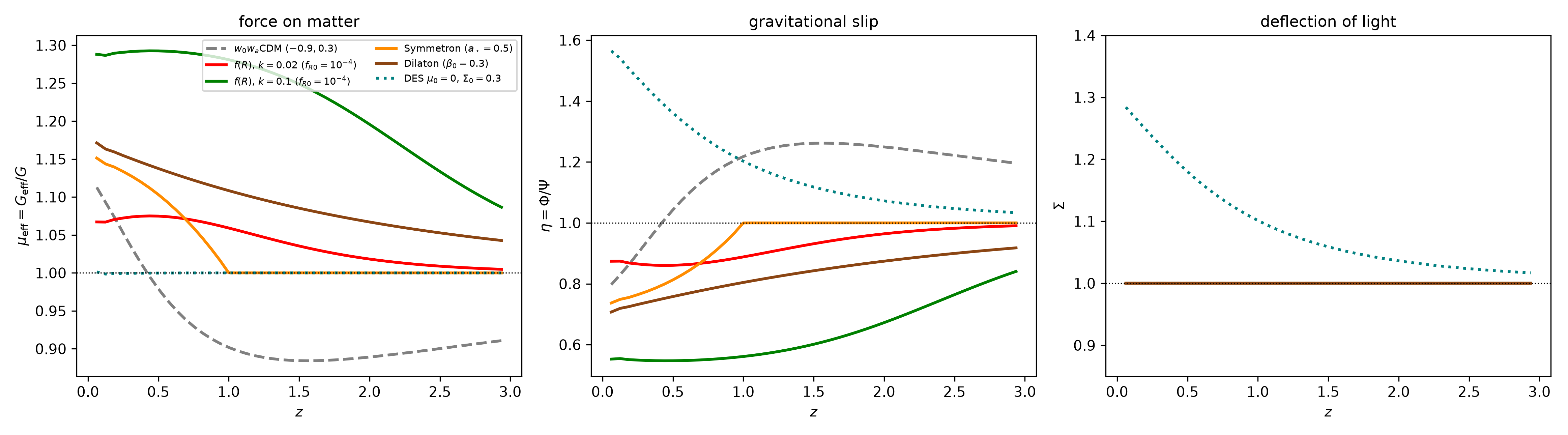
Figure 2: $\mu$, $\eta$ and $\Sigma$ for several modified gravity models including Hu-Sawicki $f(R)$ at two values of $k$, computed with MGCAMB in the associated notebook. Note that the illustrative value used there, $f_{R0}=10^{-4}$, is by now firmly excluded — it is chosen to make the effect visible.

Growth of structure

An enhancement of $\mu$ by up to $4/3$ below $\lambda_C$ translates directly into faster growth of structure on those scales, and hence a scale-dependent growth rate — something $\Lambda$CDM strictly cannot produce in the linear regime. In terms of the growth index of the cosmology class, $f\equiv\Omega_m(a)^\gamma$, one goes from $\gamma\simeq0.55$ (GR) to $\gamma\simeq0.4$ deep inside the Compton radius.

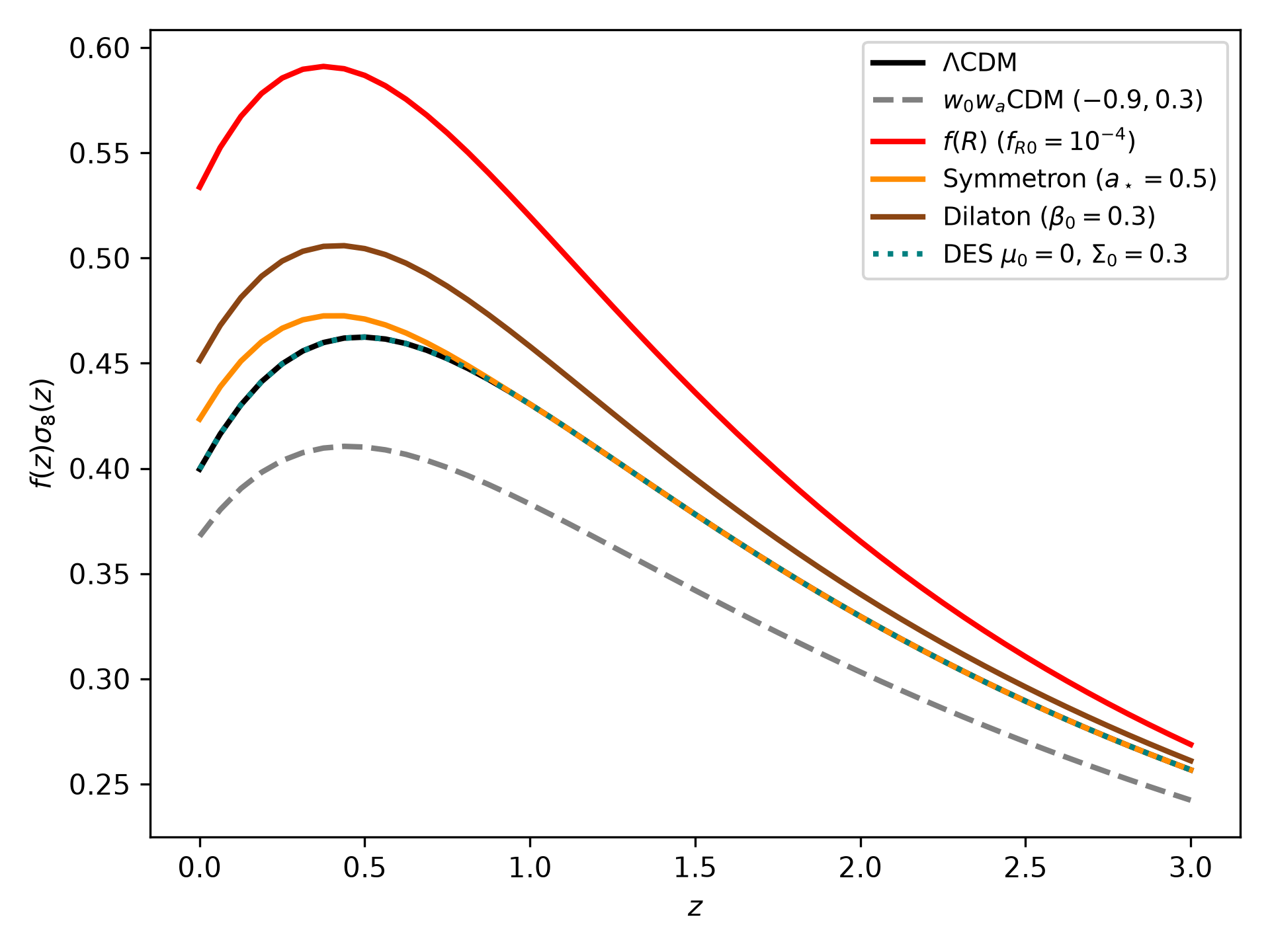
Figure 3: $f\sigma_8(z)$ for the same models. Computed in the associated notebook.

Two honest remarks about this:

It makes the $S_8$ situation worse, not better. Weak-lensing and cluster-count analyses tend to prefer less structure growth than Planck-normalised $\Lambda$CDM, whereas $f(R)$ delivers more. So $f(R)$ is not a candidate solution to the tensions of the cosmology class — the data constrain it precisely because it pushes the wrong way.
The most constraining regime is non-linear, where chameleon screening switches on inside haloes and the enhancement is suppressed in a mass-dependent way. Linear theory overestimates the signal, so quantitative constraints require $N$-body simulations (ECOSMOG, MG-GADGET, and the emulators built on them). This is why cluster abundance — sensitive to the exponential tail of the halo mass function — is such a powerful probe.

Constraints

Because screening is environment-dependent, constraints on $\vert f_{R0}\vert$ come from wildly different systems, and the least dense probes are the most powerful.

Probe	Physics	Constraint on $\vert f_{R0}\vert$ ($n=1$)
Solar system, unscreened	$\gamma=1/2$ vs Cassini	excludes the theory outright — Chiba (2003)
Milky Way self-screening	Galaxy must sit at $\Phi_N\sim10^{-6}$	$\lesssim10^{-6}$ — Hu & Sawicki (2007)
CMB + ISW, linear scales	$\mu(k)$ on Gpc scales	$\lesssim10^{-3}$ (weak: $\lambda_C$ too small to matter)
Cluster abundance	halo mass function tail	$\log_{10}\vert f_{R0}\vert<-4.79$ (95.4%) — Cataneo et al. (2015)
Cluster abundance (eRASS1)	2024 X-ray sample	$\log_{10}\vert f_{R0}\vert<-4.31$ (95%) — Artis et al. (2024)
Distance indicators in dwarfs	Cepheids vs TRGB feel different gravity	$<5\times10^{-7}$ (95%) — Jain, Vikram & Sakstein (2013)
Galaxy morphology	offset between stars and gas; warps	$<1.4\times10^{-8}$ — Desmond & Ferreira (2020)
Gravitational waves	$c_T$	no constraint: $\alpha_T=0$ exactly

Read the table from the bottom up. The tightest bound, $\vert f_{R0}\vert<1.4\times10^{-8}$, corresponds via our formula to $\lambda_C\lesssim0.4$ Mpc: the modification would be confined to sub-galactic scales. At that level $f(R)$ can no longer produce any observable cosmological effect whatsoever. As Desmond & Ferreira (2020) put it in their title, galaxy morphology rules out astrophysically relevant Hu-Sawicki $f(R)$.

The two mechanisms at work are worth distinguishing clearly:

Unscreened objects give the strongest bounds. A dwarf galaxy in a void has $\Phi_N\sim10^{-8}$ and is not screened, so it feels the full $4/3$. Compare it with an identical dwarf inside a cluster and the difference is the signal — this is the strategy we announced in the screening class, now cashed in.
Cepheids vs TRGB is a particularly elegant test: Cepheid pulsation depends on the stellar envelope, which is unscreened in an unscreened galaxy, while the tip of the red giant branch depends on the degenerate helium core, which is self-screened. Two distance indicators to the same galaxy, one modified and one not: their ratio is a direct probe of $\beta$ and $\lambda_C$, with much of the astrophysics cancelling.

Note also that constraints depend on $n$: larger $n$ makes the modification switch off faster with density, weakening the astrophysical bounds while leaving the cosmological ones roughly intact.

Looking forward, Euclid forecasts a determination of $\log_{10}\vert f_{R0}\vert$ at the $1.8\%$ level combining spectroscopic and photometric primary probes (for a fiducial $\vert f_{R0}\vert=5\times10^{-6}$), and would distinguish $\vert f_{R0}\vert=5\times10^{-7}$ from GR at more than $3\sigma$. Whether that regime is already excluded by the astrophysical bounds above is exactly the kind of cross-check that makes this field interesting: the cosmological and astrophysical constraints rely on very different systematics, and it would be unwise to trust either one alone.

And more: the rest of the higher-order landscape

$f(R)$ is the tame corner of a much wilder territory. A quick tour of what else lives under “break L3/W6”, and why each is harder:

Stelle quadratic gravity: $\mathcal{L}=R+aR^2+bR_{\mu\nu}R^{\mu\nu}$ (Stelle 1977). Power-counting renormalizable — a genuinely remarkable property for a theory of gravity — at the price of a massive spin-2 ghost. Attempts to live with it include the “fakeon” (purely virtual particle) prescription (Anselmi 2019) and the possibility that the ghost is an artefact of perturbation theory. Note that $f(R)$ is the unique subclass of quadratic gravity free of this ghost, precisely because $R^2$ alone is degenerate.
Gauss-Bonnet and Lovelock: the combination $\mathcal{G}= R^2 - 4R_{\mu\nu}R^{\mu\nu}+R_{\mu\nu\rho\sigma}R^{\mu\nu\rho\sigma}$ is topological in 4D (a total derivative, contributing nothing to the field equations), which is why it never appears in the list above. It becomes dynamical either in $D\geq5$ — that is Lovelock gravity, the subject of the higher-dimensions class — or in 4D when multiplied by a function: $f(\mathcal{G})$, or $\xi(\phi)\mathcal{G}$, which we already met as the last row of the Horndeski table (and which GW170817 has killed).
$f(R,T)$, $f(R,\mathcal{L}_m)$: let the Lagrangian depend on the matter stress tensor as well. These generically give $\nabla^\mu T_{\mu\nu}\neq0$, hence non-geodesic motion and violation of the WEP, not just the SEP. Given how strongly the WEP is tested (second class), this is a very expensive move for very little gain.
Non-local gravity: terms like $R\,\Box^{-2}R$ (Deser & Woodard 2007) or $f(R/\Box)$. The inverse d’Alembertian is not a local operator, so assumption L5 is what breaks; the theory can fit the expansion history with no free scale, but the Cauchy problem and the meaning of the boundary conditions are murky.
Infinite-derivative gravity: if a finite number of extra derivatives gives a ghost, an infinite number arranged into an entire function such as $e^{\Box/M^2}$ may not, since the propagator has no new poles. This is the ghost-free non-local gravity programme (Biswas, Mazumdar & Siegel 2005) and it is one of the more promising routes to a UV-complete gravity.
$f(T)$ and $f(Q)$: the same trick of “promote the scalar in the action to a function” applied to the torsion and non-metricity formulations of the geometric trinity. Because TEGR and STEGR are equivalent to GR but their Lagrangians differ from $R$ by a boundary term, $f(T)\neq f(R)\neq f(Q)$: the trinity is broken as soon as one goes non-linear. These are discussed in the torsion class, together with their own pathologies (broken local Lorentz invariance for $f(T)$, strongly coupled or ghostly modes for $f(Q)$).

Summary: what did we learn?

Let us step back, because the lesson of this class is more general than the theory itself.

Higher-order curvature terms are not a new road. $f(R)$ is exactly $\omega=0$ Brans-Dicke with a potential, and sits inside luminal Horndeski. We broke assumption L3 and were returned, by a Legendre transform, to a violation of L2.
The extra mode is a chameleon, necessarily. Its coupling $\beta=1/\sqrt6$ is fixed by the structure of the theory and cannot be tuned. Everything hinges on the density-dependent mass of the scalaron.
The whole phenomenology is one number, $\vert f_{R0}\vert$, equivalently one length, $\lambda_C\simeq 30\,\text{Mpc}\,(\vert f_{R0}\vert/10^{-4})^{1/2}$. Above $\lambda_C$: GR. Below: gravity is $4/3$ stronger and $\eta=1/2$.
The constraints have squeezed that length below a Megaparsec, which is to say: below any scale on which $f(R)$ was invented to do something interesting. As a dark-energy model, $f(R)$ is finished. As a benchmark — a fully worked example of a screened, scale-dependent modification with second-order equations and unmodified light propagation — it remains indispensable, and it is the model against which most survey pipelines are validated.
And $R+R^2$, at the other end of the curvature range, is a completely different story — the same function, applied at high curvature rather than low, gives our best model of inflation. That it may now be in mild tension with ACT DR6 is a reminder to keep checking.